The RELIABILITY Procedure
- Overview
-
Getting Started
 Analysis of Right-Censored Data from a Single PopulationWeibull Analysis Comparing Groups of DataAnalysis of Accelerated Life Test DataWeibull Analysis of Interval Data with Common Inspection ScheduleLognormal Analysis with Arbitrary CensoringRegression ModelingRegression Model with Nonconstant ScaleRegression Model with Two Independent VariablesWeibull Probability Plot for Two Combined Failure ModesAnalysis of Recurrence Data on RepairsComparison of Two Samples of Repair DataAnalysis of Interval Age Recurrence DataAnalysis of Binomial DataThree-Parameter WeibullParametric Model for Recurrent Events DataParametric Model for Interval Recurrent Events Data
 -
SyntaxPrimary StatementsSecondary StatementsGraphical Enhancement StatementsPROC RELIABILITY StatementANALYZE StatementBY StatementCLASS StatementDISTRIBUTION StatementEFFECTPLOT StatementESTIMATE StatementFMODE StatementFREQ StatementINSET StatementLOGSCALE StatementLSMEANS StatementLSMESTIMATE StatementMAKE StatementMCFPLOT StatementMODEL StatementNENTER StatementNLOPTIONS StatementPROBPLOT StatementRELATIONPLOT StatementSLICE StatementSTORE StatementTEST StatementUNITID Statement
-
DetailsAbbreviations and NotationTypes of Lifetime DataProbability DistributionsProbability PlottingNonparametric Confidence Intervals for Cumulative Failure ProbabilitiesParameter Estimation and Confidence IntervalsRegression Model Statistics Computed for Each Observation for Lifetime DataRegression Model Statistics Computed for Each Observation for Recurrent Events DataRecurrence Data from Repairable SystemsODS Table NamesODS Graphics
- References
Nelson (2002) and Doganaksoy and Nelson (1998) show how the difference of MCFs from two samples can be used to compare the populations from which they are drawn. The RELIABILITY procedure provides Doganaksoy and Nelson’s confidence intervals for the pointwise difference of the two MCFs, which can be used to assess whether the difference is statistically significant.
Doganaksoy and Nelson (1998) give an example of two samples of locomotives with braking grids from two different production batches. Figure 16.36 contains a listing of the data. The variable ID is a unique identifier for individual locomotives. The variable Days provides the locomotive age in days. The variable Value is 1 if the age corresponds to a braking grid replacement or -1 if the age corresponds to the locomotive’s latest age (the
current end of its history). The variable Sample is a group variable that identifies the grid production batch.
data Grids;
   if _N_ < 40 then Sample = 'Sample1';
   else Sample = 'Sample2';
   input ID$ Days Value @@;
   datalines;
S1-01 462  1    S1-01 730 -1    S1-02 364  1    S1-02 391  1
S1-02 548  1    S1-02 724 -1    S1-03 302  1    S1-03 444  1
S1-03 500  1    S1-03 730 -1    S1-04 250  1    S1-04 730 -1
S1-05 500  1    S1-05 724 -1    S1-06  88  1    S1-06 724 -1
S1-07 272  1    S1-07 421  1    S1-07 552  1    S1-07 625  1
S1-07 719 -1    S1-08 481  1    S1-08 710 -1    S1-09 431  1
S1-09 710 -1    S1-10 367  1    S1-10 710 -1    S1-11 635  1
S1-11 650  1    S1-11 708 -1    S1-12 402  1    S1-12 700 -1
S1-13  33  1    S1-13 687 -1    S1-14 287  1    S1-14 687 -1
S1-15 317  1    S1-15 498  1    S1-15 657 -1    S2-01 203  1
S2-01 211  1    S2-01 277  1    S2-01 373  1    S2-01 511 -1
S2-02 293  1    S2-02 503 -1    S2-03 173  1    S2-03 470 -1
S2-04 242  1    S2-04 464 -1    S2-05  39  1    S2-05 464 -1
S2-06  91  1    S2-06 462 -1    S2-07 119  1    S2-07 148  1
S2-07 306  1    S2-07 461 -1    S2-08 382  1    S2-08 460 -1
S2-09 250  1    S2-09 434 -1    S2-10 192  1    S2-10 448 -1
S2-11 369  1    S2-11 448 -1    S2-12  22  1    S2-12 447 -1
S2-13  54  1    S2-13 441 -1    S2-14 194  1    S2-14 432 -1
S2-15  61  1    S2-15 419 -1    S2-16  19  1    S2-16 185  1
S2-16 419 -1    S2-17 187  1    S2-17 416 -1    S2-18  93  1
S2-18 205  1    S2-18 264  1    S2-18 415 -1
;
Figure 16.36: Partial Listing of the Braking Grids Data
| Obs | Sample | ID | Days | Value |
|---|---|---|---|---|
| 1 | Sample1 | S1-01 | 462 | 1 |
| 2 | Sample1 | S1-01 | 730 | -1 |
| 3 | Sample1 | S1-02 | 364 | 1 |
| 4 | Sample1 | S1-02 | 391 | 1 |
| 5 | Sample1 | S1-02 | 548 | 1 |
| 6 | Sample1 | S1-02 | 724 | -1 |
| 7 | Sample1 | S1-03 | 302 | 1 |
| 8 | Sample1 | S1-03 | 444 | 1 |
| 9 | Sample1 | S1-03 | 500 | 1 |
| 10 | Sample1 | S1-03 | 730 | -1 |
| 11 | Sample1 | S1-04 | 250 | 1 |
| 12 | Sample1 | S1-04 | 730 | -1 |
| 13 | Sample1 | S1-05 | 500 | 1 |
| 14 | Sample1 | S1-05 | 724 | -1 |
| 15 | Sample1 | S1-06 | 88 | 1 |
| 16 | Sample1 | S1-06 | 724 | -1 |
| 17 | Sample1 | S1-07 | 272 | 1 |
| 18 | Sample1 | S1-07 | 421 | 1 |
| 19 | Sample1 | S1-07 | 552 | 1 |
| 20 | Sample1 | S1-07 | 625 | 1 |
The following statements request the Nelson (1995) nonparametric estimate and confidence limits for the difference of the MCF functions shown in Figure 16.37 for the braking grids:
proc reliability data=Grids;
   unitid ID;
   mcfplot Days*Value(-1) = Sample / mcfdiff;
run;
The MCFPLOT statement requests a plot of each MCF estimate as a function of age (provided by Days), and it specifies that the end of history for each system is identified by Value equal to -1. The variable Sample identifies the two samples of braking grids. The option MCFDIFF requests that the difference between the MCFs of the two
groups given in the variable Sample be computed and plotted. Confidence limits for the MCF difference are also computed and plotted. The UNITID statement specifies
that the variable Id uniquely identify each system.
Figure 16.37 shows the plot of the MCF difference function and pointwise 95% confidence intervals. Since the pointwise confidence limits do not include zero for some system ages, the difference between the two populations is statistically significant. A listing of the tabular output is shown in Figure 16.38. It contains a summary of the repair data for the two samples, estimates, standard errors, and confidence intervals for the MCF difference. A statistical test for different MCFs is also computed and is displayed in the table “Tests for Equality of Mean Functions.” The tests also indicate a significant difference between the two samples.
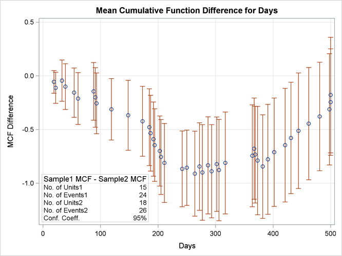
Figure 16.38: Listing of the Output for the Braking Grids Data
| MCF Difference Data Summary | |
|---|---|
| Input Data Set | WORK.GRIDS |
| Group 1 | Sample1 |
| Observations Used | 39 |
| Number of Units | 15 |
| Number of Events | 24 |
| Group 2 | Sample2 |
| Observations Used | 44 |
| Number of Units | 18 |
| Number of Events | 26 |
| Sample MCF Differences | |||||
|---|---|---|---|---|---|
| Age | MCF Difference | Standard Error | 95% Confidence Limits | Unit ID | |
| Lower | Upper | ||||
| 19.00 | -0.056 | 0.054 | -0.161 | 0.050 | S2-16 |
| 22.00 | -0.111 | 0.074 | -0.256 | 0.034 | S2-12 |
| 33.00 | -0.044 | 0.098 | -0.237 | 0.148 | S1-13 |
| 39.00 | -0.100 | 0.109 | -0.313 | 0.113 | S2-05 |
| 54.00 | -0.156 | 0.117 | -0.385 | 0.074 | S2-13 |
| 61.00 | -0.211 | 0.124 | -0.453 | 0.031 | S2-15 |
| 88.00 | -0.144 | 0.137 | -0.414 | 0.125 | S1-06 |
| 91.00 | -0.200 | 0.142 | -0.478 | 0.078 | S2-06 |
| 93.00 | -0.256 | 0.145 | -0.539 | 0.028 | S2-18 |
| 119.00 | -0.311 | 0.146 | -0.598 | -0.024 | S2-07 |
| 148.00 | -0.367 | 0.167 | -0.693 | -0.040 | S2-07 |
| 173.00 | -0.422 | 0.166 | -0.748 | -0.097 | S2-03 |
| 185.00 | -0.478 | 0.182 | -0.835 | -0.120 | S2-16 |
| 187.00 | -0.533 | 0.180 | -0.886 | -0.181 | S2-17 |
| 192.00 | -0.589 | 0.177 | -0.935 | -0.243 | S2-10 |
| 194.00 | -0.644 | 0.172 | -0.982 | -0.307 | S2-14 |
| 203.00 | -0.700 | 0.167 | -1.027 | -0.373 | S2-01 |
| 205.00 | -0.756 | 0.178 | -1.105 | -0.407 | S2-18 |
| 211.00 | -0.811 | 0.188 | -1.179 | -0.443 | S2-01 |
| 242.00 | -0.867 | 0.180 | -1.219 | -0.514 | S2-04 |
| 250.00 | -0.856 | 0.179 | -1.207 | -0.504 | S1-04,S2-09 |
| 264.00 | -0.911 | 0.202 | -1.307 | -0.515 | S2-18 |
| 272.00 | -0.844 | 0.208 | -1.252 | -0.437 | S1-07 |
| 277.00 | -0.900 | 0.227 | -1.345 | -0.455 | S2-01 |
| 287.00 | -0.833 | 0.231 | -1.286 | -0.380 | S1-14 |
| 293.00 | -0.889 | 0.222 | -1.323 | -0.455 | S2-02 |
| 302.00 | -0.822 | 0.224 | -1.262 | -0.383 | S1-03 |
| 306.00 | -0.878 | 0.241 | -1.350 | -0.406 | S2-07 |
| 317.00 | -0.811 | 0.242 | -1.286 | -0.337 | S1-15 |
| 364.00 | -0.744 | 0.242 | -1.219 | -0.270 | S1-02 |
| 367.00 | -0.678 | 0.241 | -1.150 | -0.206 | S1-10 |
| 369.00 | -0.733 | 0.230 | -1.185 | -0.282 | S2-11 |
| 373.00 | -0.789 | 0.257 | -1.293 | -0.284 | S2-01 |
| 382.00 | -0.844 | 0.246 | -1.327 | -0.362 | S2-08 |
| 391.00 | -0.778 | 0.261 | -1.290 | -0.266 | S1-02 |
| 402.00 | -0.711 | 0.258 | -1.217 | -0.206 | S1-12 |
| 421.00 | -0.644 | 0.270 | -1.174 | -0.115 | S1-07 |
| 431.00 | -0.578 | 0.265 | -1.097 | -0.059 | S1-09 |
| 444.00 | -0.511 | 0.275 | -1.049 | 0.027 | S1-03 |
| 462.00 | -0.444 | 0.267 | -0.968 | 0.079 | S1-01 |
| 481.00 | -0.378 | 0.258 | -0.883 | 0.128 | S1-08 |
| 498.00 | -0.311 | 0.265 | -0.830 | 0.208 | S1-15 |
| 500.00 | -0.244 | 0.253 | -0.741 | 0.252 | S1-05 |
| 500.00 | -0.178 | 0.275 | -0.716 | 0.360 | S1-03 |
| Tests for Equality of Mean Cumulative Functions | |||||
|---|---|---|---|---|---|
| Weight Function | Statistic | Variance | Chi Square | DF | Pr > Chi Square |
| Constant | -3.673285 | 4.556053 | 2.961560 | 1 | 0.0853 |
| Linear | -4.435032 | 1.424770 | 13.805393 | 1 | 0.0002 |
You can fit a parametric model that uses Sample as a classification variable. This results in a model with a common shape parameter for the two groups but with different
scale parameters. Suppose you want estimates of the parametric mean and intensity functions at values of the time variable
500, 600, 700, 800, 900, and 1,000 days for each of the two groups. The following statements create a new input data set that
has observations for the desired prediction times appended to it. The additional observations are not used in the analysis,
because the censoring variable Value is set to missing for those observations. Values of the mean and intensity function are computed, however, in the table that
is produced by specifying the OBSTATS option in the MODEL statement.
The following statements create the new data set by appending observations to the original Grids data set:
data Predict;
   Control=1;
   if _N_ < 7 then Sample = 'Sample1';
   else Sample = 'Sample2';

   input ID$ Days Value;
   cards;
9999 500  .
9999 600  .
9999 700  .
9999 800  .
9999 900  .
9999 1000 .
9999 500  .
9999 600  .
9999 700  .
9999 800  .
9999 900  .
9999 1000 .
;

data Grids;
   set Predict Grids;
run;
The following statements fit a nonhomogeneous Poisson process with a power law mean function that uses Sample as a two-level covariate. The OBSTATS option requests that predicted values be computed for values of the variable Control equal to 1. The MCFPLOT statement plots the fitted model as well as the nonparametric estimates of the MCF. Parametric confidence
limits are displayed by default.
proc reliability data=Grids;
   unitid ID;
   distribution nhpp(pow);
   class Sample;
   model   Days*Value(-1) = Sample /obstats(control=Control);
   mcfplot Days*Value(-1) = Sample /fit=model overlay;
run;
Figure 16.39: Predicted Mean and Intensity Function for the Braking Grids Data
| Observation Statistics | |||||||||||||
|---|---|---|---|---|---|---|---|---|---|---|---|---|---|
| Days | Value | Sample | ID | Xbeta | Shape | MCF | MCF_Lower | MCF_Upper | MCF_StdErr | Intensity | Int_Lower | Int_Upper | Int_StdErr |
| 500 | . | Sample1 | 9999 | 464.04648 | 1.1050556 | 1.0859585 | 0.7176451 | 1.6432995 | 0.2295199 | 0.0024001 | 0.0015543 | 0.0037061 | 0.000532 |
| 600 | . | Sample1 | 9999 | 464.04648 | 1.1050556 | 1.3283512 | 0.8874029 | 1.9884054 | 0.2733977 | 0.0024465 | 0.0015458 | 0.0038719 | 0.0005731 |
| 700 | . | Sample1 | 9999 | 464.04648 | 1.1050556 | 1.5750445 | 1.0556772 | 2.3499278 | 0.3215248 | 0.0024864 | 0.0015325 | 0.0040343 | 0.000614 |
| 800 | . | Sample1 | 9999 | 464.04648 | 1.1050556 | 1.8254803 | 1.2215469 | 2.7279987 | 0.3741606 | 0.0025216 | 0.0015171 | 0.0041911 | 0.0006537 |
| 900 | . | Sample1 | 9999 | 464.04648 | 1.1050556 | 2.0792348 | 1.3846219 | 3.1223089 | 0.4313142 | 0.002553 | 0.0015011 | 0.0043418 | 0.0006917 |
| 1000 | . | Sample1 | 9999 | 464.04648 | 1.1050556 | 2.3359745 | 1.5448083 | 3.5323327 | 0.4928631 | 0.0025814 | 0.0014852 | 0.0044866 | 0.000728 |
| 500 | . | Sample2 | 9999 | 323.23791 | 1.1050556 | 1.6193855 | 1.1012136 | 2.3813813 | 0.3186232 | 0.003579 | 0.0021872 | 0.0058566 | 0.0008993 |
| 600 | . | Sample2 | 9999 | 323.23791 | 1.1050556 | 1.9808425 | 1.335699 | 2.9375905 | 0.3982653 | 0.0036482 | 0.0021492 | 0.0061928 | 0.0009849 |
| 700 | . | Sample2 | 9999 | 323.23791 | 1.1050556 | 2.3487125 | 1.5633048 | 3.5287107 | 0.4878045 | 0.0037078 | 0.0021124 | 0.006508 | 0.0010643 |
| 800 | . | Sample2 | 9999 | 323.23791 | 1.1050556 | 2.7221634 | 1.7845232 | 4.1524669 | 0.5864921 | 0.0037602 | 0.002078 | 0.0068042 | 0.0011378 |
| 900 | . | Sample2 | 9999 | 323.23791 | 1.1050556 | 3.100563 | 2.0000301 | 4.8066733 | 0.6935604 | 0.003807 | 0.002046 | 0.0070837 | 0.0012061 |
| 1000 | . | Sample2 | 9999 | 323.23791 | 1.1050556 | 3.4834144 | 2.2104841 | 5.4893747 | 0.8083117 | 0.0038494 | 0.0020164 | 0.0073484 | 0.0012699 |
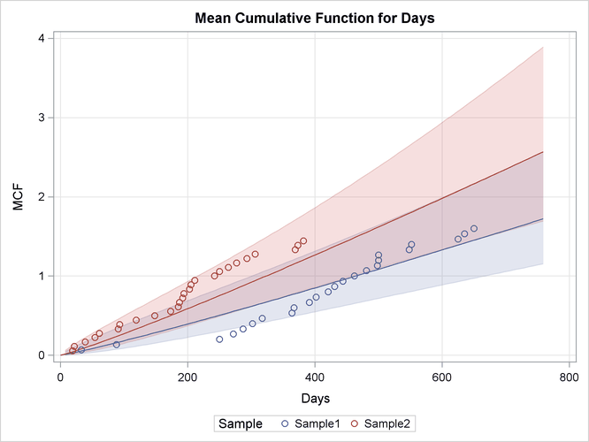
The predicted values of the mean and intensity functions at the desired values of Days, with standard errors and confidence limits, are shown in Figure 16.39.
A plot of the fitted mean function, along with nonparametric estimates for the two samples, is shown in Figure 16.40.