The MVPMODEL Procedure

To build a model that has only three principal components, you can use the NCOMP= option as shown in the following statements:
proc mvpmodel data=MWflightDelays ncomp=3 plots=(all score(labels=on))
              out=outDelays;
   var AA CO DL F9 FL NW UA US WN;
run;
The PLOTS=ALL option requests all possible plots, which include pairwise plots of the principal component scores and loadings in addition
to the default scree plot and variance-explained plot. The OUT= option produces an output data set called outDelays that contains principal component scores, ![]() statistics, SPE statistics, residuals, and more, as described in the section Output Data Sets. Note that ODS Graphics is still enabled, so you do not need to specify the ODS GRAPHICS ON statement here.
statistics, SPE statistics, residuals, and more, as described in the section Output Data Sets. Note that ODS Graphics is still enabled, so you do not need to specify the ODS GRAPHICS ON statement here.
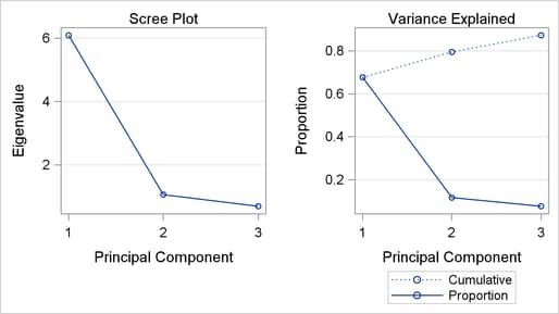
The correlation matrix is the same as in Figure 12.2. The eigenvalue information, scree plot, and variance-explained plot are similar to those in Figure 12.3 and Figure 12.4. However, the use of the NCOMP=3 option results in outputs that show information only for the three components in the model, as seen in Figure 12.5 and Figure 12.6.
Figure 12.5: Eigenvalue and Variance Information
| Eigenvalues of the Correlation Matrix | ||||
|---|---|---|---|---|
| Eigenvalue | Difference | Proportion | Cumulative | |
| 1 | 6.09006397 | 5.02872938 | 0.6767 | 0.6767 |
| 2 | 1.06133459 | 0.36642409 | 0.1179 | 0.7946 |
| 3 | 0.69491050 | 0.0772 | 0.8718 | |
Also, the model summary, shown in Figure 12.7, is different because there are now only three principal components in the model.
Figure 12.7: Summary of Model and Data Information
| Data Set | WORK.MWFLIGHTDELAYS |
|---|---|
| Number of Variables | 9 |
| Missing Value Handling | Exclude |
| Number of Observations Read | 16 |
| Number of Observations Used | 16 |
| Number of Principal Components | 3 |
The outDelays output data set that is partially listed in Figure 12.8 contains ![]() and SPE statistics based on the model that has three principal components, in addition to the original variables and other
observationwise statistics.
and SPE statistics based on the model that has three principal components, in addition to the original variables and other
observationwise statistics.
Figure 12.8: Partial Listing of Output Data Set outDelays
| flightDate | AA | CO | DL | F9 | FL | NW | UA | US | WN | Prin1 | Prin2 | Prin3 | _NOBS_ | _TSQUARE_ | R_AA | R_CO | R_DL | R_F9 | R_FL | R_NW | R_UA | R_US | R_WN | _SPE_ |
|---|---|---|---|---|---|---|---|---|---|---|---|---|---|---|---|---|---|---|---|---|---|---|---|---|
| 02/01/07 | 14.9 | 7.1 | 7.9 | 8.5 | 14.8 | 4.5 | 5.1 | 13.4 | 5.1 | -1.08708 | 1.20953 | -0.03839 | 16 | 1.57457 | -0.05779 | -0.18178 | -0.01835 | -0.15280 | 0.87457 | -0.37864 | -0.06037 | -0.12896 | -0.02300 | 0.98911 |
| 02/02/07 | 14.3 | 9.6 | 14.1 | 6.2 | 12.8 | 6.0 | 3.9 | 15.3 | 11.4 | -0.65786 | 1.26249 | 0.11447 | 16 | 1.59169 | -0.17802 | -0.16663 | 0.68047 | -0.62682 | 0.49289 | -0.35101 | -0.27027 | -0.14161 | 0.41169 | 1.54414 |
| 02/03/07 | 23.0 | 6.1 | 1.7 | 0.9 | 11.9 | 15.2 | 9.5 | 18.4 | 7.6 | -0.86457 | -0.73183 | 0.29270 | 16 | 0.75065 | 0.54274 | -0.30297 | -0.20552 | -0.02408 | 0.31360 | 0.21270 | -0.49772 | 0.24287 | -0.23829 | 0.93626 |
| 02/04/07 | 6.5 | 6.3 | 3.9 | -0.2 | 8.4 | 18.8 | 6.2 | 8.8 | 8.0 | -1.50578 | -0.69718 | 1.32511 | 16 | 3.35709 | -0.25729 | -0.24974 | 0.05624 | 0.05279 | -0.02427 | 0.29305 | -0.44076 | 0.13493 | 0.50899 | 0.69253 |
| 02/05/07 | 12.0 | 14.1 | 3.3 | -1.3 | 10.0 | 13.1 | 22.8 | 16.5 | 11.5 | -0.63903 | -1.11141 | 0.38617 | 16 | 1.44549 | -0.44128 | 0.28274 | 0.09998 | -0.15050 | 0.00176 | -0.36866 | 0.39124 | 0.07233 | -0.06265 | 0.60545 |
The variables Prin1, Prin2, and Prin3 contain the principal component scores. Variables R_AA through R_WN are the residuals for the process variables. The contents of an OUT= data set are described in detail in the section Output Data Sets. See the section Principal Component Analysis for computational details of the results saved in the output data set.
You can use an OUT= data set as an input to the MVPMONITOR and MVPDIAGNOSE procedures. The MVPMONITOR procedure produces control
charts for the ![]() and SPE statistics. Control charts that are created from the
and SPE statistics. Control charts that are created from the outDelays data set are shown in Example 12.2 and in the MVPMONITOR procedure chapter.
The PLOTS=ALL option produces score plots for pairs of principal components in the model. By default, the score plots are displayed in a matrix. You can specify the PLOTS(SCORES(UNPACK)) option to display the score plots as separate graphs. The score plot matrix is shown in Figure 12.9.
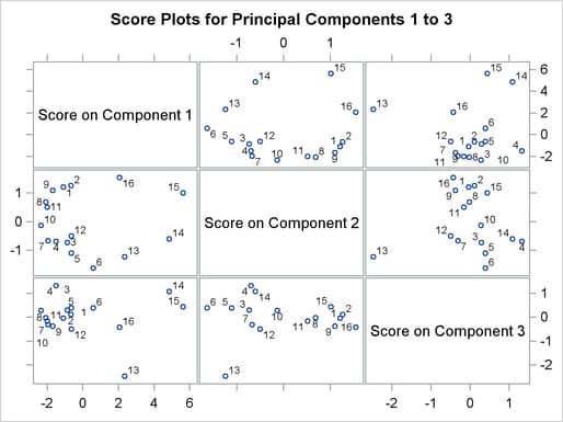
A score plot is a scatter plot of the scores for two principal components. The labels indicate the observation numbers of the points. By examining clusters and outliers in these plots, you can better understand the relationships among the observations and the variation in the process. For example, points 13 through 16 are extreme points in the direction of the first principal component. The directions of the principal components are not uniquely determined, so you need the loadings and external information to interpret them. These points represent flight delays between February 13, 2007, and February 16, 2007, when there was a major winter storm in the Midwest.
Figure 12.10 displays the loading plots that are produced. Loading plots are also displayed in a matrix by default, and they can be unpacked into separate graphs with the PLOT(LOADINGS(UNPACK)) option.
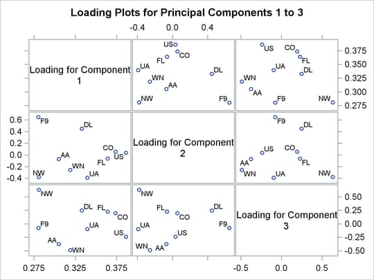
A loading plot is a scatter plot of the variable loadings for a pair of principal components, and it helps you understand
the relationships among the variables. Loadings are the variable coefficients in the eigenvectors (linear combinations of
variables) that define the principal component. The loadings explain how variables contribute to the linear combination. Here,
the loadings for the first principal component are all positive and all similar in value, which suggests that the first principal
component describes the average delay. The second principal component appears to be a contrast between the delays of F9, DL, CO, and US and those of the remaining airlines. See the section Principal Component Analysis for more information about interpreting principal component loadings and scores.