XCHART Statement: CUSUM Procedure

Example 6.1 Cusum and Standard Deviation Charts

See CUSXS in the SAS/QC Sample LibraryWhen you are working with subgrouped data, it can be helpful to accompany a cusum chart for means with a Shewhart s chart for monitoring the variability of the process. This example creates this combination for the variable Weight in the data set Oil (see Creating a V-Mask Cusum Chart from Raw Data).

The first step is to create a one-sided cusum chart for means that detects a shift of one standard error ( $\delta =-1$ ) below the target mean.

proc cusum data=Oil;
   xchart Weight*Hour /
      nochart
      mu0=8.100        /* target mean for process  */
      sigma0=0.050     /* known standard deviation */
      delta=-1         /* shift to be detected     */
      h=3              /* cusum parameter h        */
      k=0.5            /* cusum parameter k        */
      scheme=onesided
      outtable = Tabcusum
         ( drop   = _var_ _subn_ _subx_ _exlim_
           rename = ( _cusum_ = _subx_ _h_ = _uclx_ ) )
      ;
run;

The results are saved in an OUTTABLE= data set named Tabcusum. The cusum variable (_CUSUM_) and the decision interval variable (_H_) are renamed to _SUBX_ and _LCLX_ so that they can later be read by the SHEWHART procedure.

The next step is to construct a Shewhart $\bar{X}$ and s chart for Weight and save the results in a data set named Tabxscht.

proc shewhart data=Oil;
   xschart Weight*Hour /
      nochart
      outtable = Tabxscht
         ( drop = _subx_  _uclx_ );
run;

Note that the variables _SUBX_ and _UCLX_ are dropped from Tabxscht.

The third step is to merge the data sets Tabcusum and Tabxscht.

data taball;
   merge Tabxscht Tabcusum; by Hour;
   _mean_ = _uclx_ * 0.5;
   _lclx_ = 0.0;
run;

The variable _LCLX_ is assigned the role of the lower limit for the cusums, and the variable _MEAN_ is assigned a dummy value. Now, TABALL, which is listed in Output 6.1.1, has the structure required for a TABLE= data set used with the XSCHART statement in the SHEWHART procedure (see TABLE= Data Set).

Output 6.1.1: Listing of the Data Set TABALL

Obs	_VAR_	Hour	_SIGMAS_	_LIMITN_	_SUBN_	_MEAN_	_STDDEV_	_SUBS_	_S_	_UCLS_	_subx_	_uclx_
1	Weight	1	3	4	4	1.5	0.05	0.059640	0.049943	0.11317	0.00	3
2	Weight	2	3	4	4	1.5	0.05	0.090220	0.049943	0.11317	0.00	3
3	Weight	3	3	4	4	1.5	0.05	0.076346	0.049943	0.11317	0.00	3
4	Weight	4	3	4	4	1.5	0.05	0.025552	0.049943	0.11317	0.00	3
5	Weight	5	3	4	4	1.5	0.05	0.026500	0.049943	0.11317	0.00	3
6	Weight	6	3	4	4	1.5	0.05	0.075617	0.049943	0.11317	0.30	3
7	Weight	7	3	4	4	1.5	0.05	0.037242	0.049943	0.11317	0.00	3
8	Weight	8	3	4	4	1.5	0.05	0.059290	0.049943	0.11317	0.18	3
9	Weight	9	3	4	4	1.5	0.05	0.005737	0.049943	0.11317	1.21	3
10	Weight	10	3	4	4	1.5	0.05	0.046522	0.049943	0.11317	0.62	3
11	Weight	11	3	4	4	1.5	0.05	0.040542	0.049943	0.11317	0.00	3
12	Weight	12	3	4	4	1.5	0.05	0.056103	0.049943	0.11317	0.00	3

The final step is to use the SHEWHART procedure to read TABALL as a TABLE= data set and to display the cusum and s charts.

ods graphics off;
symbol v=dot color=salmon h=1.8 pct;
title 'Cusum Chart for Mean and s chart';
proc shewhart table=taball;
   xschart Weight * Hour /
      nolimitslegend
      ucllabel = 'h=3.0'
      noctl
      split = '/'
      nolegend ;
   label _subx_ = 'Lower Cusum/Std Dev';
run;

The central line for the primary (cusum) chart is suppressed with the NOCTL option, and the default 3 $\sigma$ Limits legend is suppressed with the NOLIMITLEGEND option. The charts are shown in Output 6.1.2.

Output 6.1.2: Combined Cusum Chart and s Chart

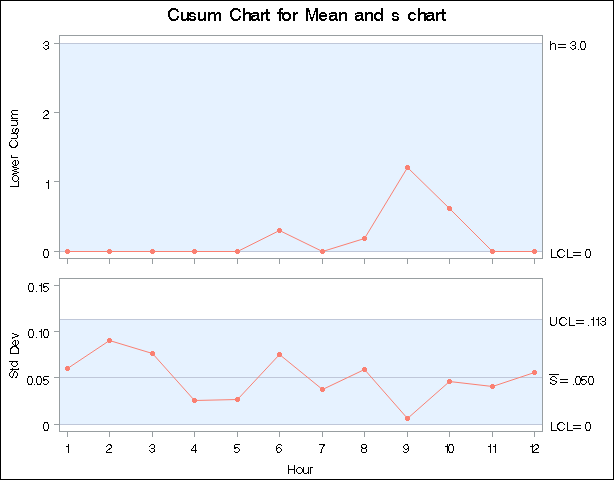
The process variability is stable, and there is no signal of a downward shift in the process mean.