QQPLOT Statement: CAPABILITY Procedure
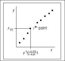
Figure 5.43 illustrates how a Q-Q plot is constructed. First, the n nonmissing values of the variable are ordered from smallest to largest:
![]()
Then the ith ordered value ![]() is represented on the plot by a point whose y-coordinate is
is represented on the plot by a point whose y-coordinate is ![]() and whose x-coordinate is
and whose x-coordinate is ![]() , where
, where ![]() is the theoretical distribution with zero location parameter and unit scale parameter.
is the theoretical distribution with zero location parameter and unit scale parameter.
You can modify the adjustment constants –0.375 and 0.25 with the RANKADJ= and NADJ= options. This default combination is recommended by Blom (1958). For additional information, refer to Chambers et al. (1983). Since ![]() is a quantile of the empirical cumulative distribution function (ecdf), a Q-Q plot compares quantiles of the ecdf with quantiles
of a theoretical distribution. Probability plots (see PROBPLOT Statement: CAPABILITY Procedure) are constructed the same way, except that the x-axis is scaled nonlinearly in percentiles.
is a quantile of the empirical cumulative distribution function (ecdf), a Q-Q plot compares quantiles of the ecdf with quantiles
of a theoretical distribution. Probability plots (see PROBPLOT Statement: CAPABILITY Procedure) are constructed the same way, except that the x-axis is scaled nonlinearly in percentiles.

