Tests for Normality :: SAS/QC(R) 12.3 User's Guide

Tests for Normality

You can use the NORMALTEST option in the PROC CAPABILITY statement to request several tests of the hypothesis that the analysis variable values are a random sample from a normal distribution. These tests, which are summarized in the table labeled Tests for Normality, include the following:

Shapiro-Wilk test
Kolmogorov-Smirnov test
Anderson-Darling test
Cramér-von Mises test

Tests for normality are particularly important in process capability analysis because the commonly used capability indices are difficult to interpret unless the data are at least approximately normally distributed. Furthermore, the confidence limits for capability indices displayed in the table labeled Process Capability Indices require the assumption of normality. Consequently, the tests of normality are always computed when you specify the SPEC statement, and a note is added to the table when the hypothesis of normality is rejected. You can specify the particular test and the significance level with the CHECKINDICES option.

Shapiro-Wilk Test

If the sample size is 2000 or less, [16] the procedure computes the Shapiro-Wilk statistic W (also denoted as to emphasize its dependence on the sample size n). The statistic is the ratio of the best estimator of the variance (based on the square of a linear combination of the order statistics) to the usual corrected sum of squares estimator of the variance. When n is greater than three, the coefficients to compute the linear combination of the order statistics are approximated by the method of Royston (1992). The statistic is always greater than zero and less than or equal to one $(0 < W \leq 1)$ .

Small values of W lead to rejection of the null hypothesis. The method for computing the p-value (the probability of obtaining a W statistic less than or equal to the observed value) depends on n. For n = 3, the probability distribution of W is known and is used to determine the p-value. For n > 4, a normalizing transformation is computed:

$\displaystyle Z_{n} = \left\{ \begin{array}{ll} ( - \log ( \gamma - \log ( 1- W_ n ) ) - \mu ) / \sigma & \mbox{if $4 \leq n \leq 11 $} \\ ( \log ( 1 - W_ n ) - \mu ) / \sigma & \mbox{if $12 \leq n \leq 2000 $} \end{array} \right.$

The values of $\sigma$ , $\gamma$ , and $\mu$ are functions of n obtained from simulation results. Large values of indicate departure from normality, and since the statistic has an approximately standard normal distribution, this distribution is used to determine the p-values for n > 4.

EDF Tests for Normality

The Kolmogorov-Smirnov, Anderson-Darling and Cramér-von Mises tests for normality are based on the empirical distribution function (EDF) and are often referred to as EDF tests. EDF tests for a variety of non-normal distributions are available in the HISTOGRAM statement; see the section EDF Goodness-of-Fit Tests for details. For a thorough discussion of these tests, refer to D’Agostino and Stephens (1986).

The empirical distribution function is defined for a set of n independent observations $X_1,\ldots ,X_ n$ with a common distribution function . Under the null hypothesis, is the normal distribution. Denote the observations ordered from smallest to largest as $X_{(1)},\ldots ,X_{(n)}$ . The empirical distribution function, , is defined as

$\displaystyle F_{n}(x) = \left\{ \begin{array}{ll} 0, & x < X_{(1)} \\ \frac{i}{n}, & X_{(i)} \leq x < X_{(i+1)} , i=1,\ldots ,n-1 \\ 1, & X_{(n)} \leq x \end{array} \right.$

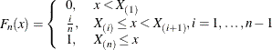Note that is a step function that takes a step of height $\frac{1}{n}$ at each observation. This function estimates the distribution function . At any value x, is the proportion of observations less than or equal to x, while is the probability of an observation less than or equal to x. EDF statistics measure the discrepancy between and .

The EDF tests make use of the probability integral transformation . If is the distribution function of X, the random variable U is uniformly distributed between 0 and 1. Given n observations $X_{(1)},\ldots ,X_{(n)}$ , the values $U_{(i)}=F(X_{(i)})$ are computed. These values are used to compute the EDF test statistics, as described in the next three sections. The CAPABILITY procedures computes the associated p-values by interpolating internal tables of probability levels similar to those given by D’Agostino and Stephens (1986).

Kolmogorov-Smirnov Test

The Kolmogorov-Smirnov statistic (D) is defined as

$D = \mbox{sup}_ x|F_{n}(x)-F(x)|$

The Kolmogorov-Smirnov statistic belongs to the supremum class of EDF statistics. This class of statistics is based on the largest vertical difference between and .

The Kolmogorov-Smirnov statistic is computed as the maximum of $D^{+}$ and $D^{-}$ , where $D^{+}$ is the largest vertical distance between the EDF and the distribution function when the EDF is greater than the distribution function, and $D^{-}$ is the largest vertical distance when the EDF is less than the distribution function.

$\begin{array}{lll} D^{+} & = & \max _{i}\left(\frac{i}{n} - U_{(i)}\right) \\ D^{-} & = & \max _{i}\left(U_{(i)} - \frac{i-1}{n}\right) \\ D & = & \max \left(D^{+},D^{-}\right) \end{array}$

PROC CAPABILITY uses a modified Kolmogorov D statistic to test the data against a normal distribution with mean and variance equal to the sample mean and variance.

Anderson-Darling Test

The Anderson-Darling statistic and the Cramér-von Mises statistic belong to the quadratic class of EDF statistics. This class of statistics is based on the squared difference $\left(F_ n(x)- F(x)\right)^2$ . Quadratic statistics have the following general form:

$Q = n \int _{-\infty }^{+\infty } \left(F_ n(x)-F(x)\right)^2 \psi (x) dF(x)$

The function $\psi (x)$ weights the squared difference $\left(F_ n(x)- F(x)\right)^2$ .

The Anderson-Darling statistic () is defined as

$A^{2} = n\int _{-\infty }^{+\infty }\left(F_ n(x)-F(x)\right)^2 \left[F(x)\left(1-F(x)\right)\right]^{-1} dF(x)$

Here the weight function is $\psi (x) = \left[F(x)\left(1-F(x)\right)\right]^{-1}$ .

The Anderson-Darling statistic is computed as

$A^2 = -n-\frac{1}{n}\sum _{i=1}^ n \left[(2i-1)\log U_{(i)} + (2n+1-2i) \log \left(\{ 1-U_{(i)}\right)\right]$

Cramér-von Mises Test

The Cramér-von Mises statistic () is defined as

$W^2 = n \int _{-\infty }^{+\infty } \left(F_{n}(x)-F(x)\right)^2 dF(x)$

Here the weight function is $\psi (x) = 1$ .

The Cramér-von Mises statistic is computed as

$W^2 = \sum _{i=1}^ n\left(U_{(i)}-\frac{2i-1}{2n}\right)^2 + \frac{1}{12n}$

^[16]In SAS 6.12 and earlier releases, the CAPABILITY procedure performed a Shapiro-Wilk test for sample sizes of 2000 or smaller, and a Kolmogorov-Smirnov test otherwise. The computed value of W was used to interpolate linearly within the range of simulated critical values given in Shapiro and Wilk (1965). In SAS 7, minor improvements were made to the algorithm for the Shapiro-Wilk test, as described in this section.