PROBPLOT Statement: CAPABILITY Procedure

Example 5.20 Displaying a Lognormal Reference Line
See CAPPROB3 in the SAS/QC Sample LibraryThis example is a continuation of Creating Lognormal Probability Plots. Figure 5.36 shows that a lognormal distribution with shape parameter ![]() is a good fit for the distribution of
is a good fit for the distribution of Diameter in the data set Rods.
The lognormal distribution involves two other parameters: a threshold parameter ![]() and a scale parameter
and a scale parameter ![]() . See Table 5.62 for the equation of the lognormal density function. The following statements illustrate how you can request a diagonal distribution
reference line whose slope and intercept are determined by estimates of
. See Table 5.62 for the equation of the lognormal density function. The following statements illustrate how you can request a diagonal distribution
reference line whose slope and intercept are determined by estimates of ![]() and
and ![]() .
.
ods graphics off;
symbol v=plus height=3.5pct;
title 'Lognormal Probability Plot for Diameters';
proc capability data=Rods noprint;
   probplot Diameter / lognormal(sigma=0.5 theta=est zeta=est)
                       square
                       pctlminor
                       href      = 95
                       hreflabel = '95%'
                       vref      = 5.8 to 6.0 by 0.1
                       chref     = red
                       cvref     = blue;
run;
The plot is shown in Output 5.20.1.
Output 5.20.1: Lognormal Reference Line
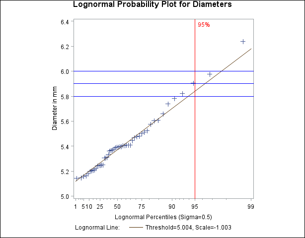
The close agreement between the diagonal reference line and the point pattern indicates that the specific lognormal distribution
with ![]() ,
, ![]() , and
, and ![]() is a good fit for the diameter measurements.
is a good fit for the diameter measurements.
Specifying HREF=95 adds a reference line indicating the 95th percentile of the lognormal distribution. The HREFLABEL= option specifies a label for this line. The PCTLMINOR option displays minor tick marks on the percentile axis. The VREF= option adds reference lines indicating diameter values of 5.8, 5.9, and 6.0, and the CHREF= and CVREF= options specify colors for the horizontal and vertical reference lines.
Based on the intersection of the diagonal reference line with the HREF= line, the estimated 95th percentile of the diameter distribution is 5.85 mm.
Note that you could also construct a similar plot in which all three parameters are estimated by substituting SIGMA=EST for SIGMA=0.5 in the preceding statements.