Calculating the Chart Statistic
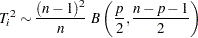
In this situation, it was shown by Gnanadesikan and Kettenring (1972), using a result of Wilks (1962), that  is exactly distributed as a multiple of a variable with a beta distribution. Specifically,
 |
Tracy, Young, and Mason (1992) used this result to derive initial control limits for a multivariate chart based on three quality measures from a chemical process in the start-up phase: percent of impurities, temperature, and concentration. The remainder of this section describes the construction of a multivariate control chart using their data, which are given here by the data set Startup.
data Startup;
   input Sample Impure Temp Conc;
   label Sample = 'Sample Number'
         Impure = 'Impurities'
         Temp   = 'Temperature'
         Conc   = 'Concentration' ;
   datalines;
 1  14.92  85.77  42.26
 2  16.90  83.77  43.44
 3  17.38  84.46  42.74
 4  16.90  86.27  43.60
 5  16.92  85.23  43.18
 6  16.71  83.81  43.72
 7  17.07  86.08  43.33
 8  16.93  85.85  43.41
 9  16.71  85.73  43.28
10  16.88  86.27  42.59
11  16.73  83.46  44.00
12  17.07  85.81  42.78
13  17.60  85.92  43.11
14  16.90  84.23  43.48
;
In preparation for the computation of the control limits, the sample size is calculated and parameter variables are defined.
proc means data=Startup noprint ;
   var Impure Temp Conc;
   output out=means n=n;
run;

data Startup;
   if _n_ = 1 then set means;
   set Startup;
   p        = 3;
   _subn_   = 1;
   _limitn_ = 1;
run;
Next, the PRINCOMP procedure is used to compute the principal components of the variables and save them in an output data set named Prin.
proc princomp data=Startup out=Prin outstat=scores std cov;
   var Impure Temp Conc;
run;
The following statements compute and its exact control limits, using the fact that is the sum of squares of the principal components.1 Note that these statements create several special SAS variables so that the data set Prin can subsequently be read as a TABLE= input data set by the SHEWHART procedure. These special variables begin and end with an underscore character. The data set Prin is listed in Figure 15.222.
data Prin (rename=(tsquare=_subx_));
   length _var_ $ 8 ;
   drop prin1 prin2 prin3 _type_ _freq_;
   set Prin;
   comp1   = prin1*prin1;
   comp2   = prin2*prin2;
   comp3   = prin3*prin3;
   tsquare = comp1 + comp2 + comp3;
   _var_   = 'tsquare';
   _alpha_ = 0.05;
   _lclx_  = ((n-1)*(n-1)/n)*betainv(_alpha_/2, p/2, (n-p-1)/2);
   _mean_  = ((n-1)*(n-1)/n)*betainv(0.5, p/2, (n-p-1)/2);
   _uclx_  = ((n-1)*(n-1)/n)*betainv(1-_alpha_/2, p/2, (n-p-1)/2);
   label tsquare = 'T Squared'
         comp1   = 'Comp 1'
         comp2   = 'Comp 2'
         comp3   = 'Comp 3';
run;
| T2 Chart For Chemical Example |
| _var_ | n | Sample | Impure | Temp | Conc | p | _subn_ | _limitn_ | comp1 | comp2 | comp3 | _subx_ | _alpha_ | _lclx_ | _mean_ | _uclx_ |
|---|---|---|---|---|---|---|---|---|---|---|---|---|---|---|---|---|
| tsquare | 14 | 1 | 14.92 | 85.77 | 42.26 | 3 | 1 | 1 | 0.79603 | 10.1137 | 0.01606 | 10.9257 | 0.05 | 0.24604 | 2.44144 | 7.13966 |
| tsquare | 14 | 2 | 16.90 | 83.77 | 43.44 | 3 | 1 | 1 | 1.84804 | 0.0162 | 0.17681 | 2.0410 | 0.05 | 0.24604 | 2.44144 | 7.13966 |
| tsquare | 14 | 3 | 17.38 | 84.46 | 42.74 | 3 | 1 | 1 | 0.33397 | 0.1538 | 5.09491 | 5.5827 | 0.05 | 0.24604 | 2.44144 | 7.13966 |
| tsquare | 14 | 4 | 16.90 | 86.27 | 43.60 | 3 | 1 | 1 | 0.77286 | 0.3289 | 2.76215 | 3.8640 | 0.05 | 0.24604 | 2.44144 | 7.13966 |
| tsquare | 14 | 5 | 16.92 | 85.23 | 43.18 | 3 | 1 | 1 | 0.00147 | 0.0165 | 0.01919 | 0.0372 | 0.05 | 0.24604 | 2.44144 | 7.13966 |
| tsquare | 14 | 6 | 16.71 | 83.81 | 43.72 | 3 | 1 | 1 | 1.91534 | 0.0645 | 0.27362 | 2.2534 | 0.05 | 0.24604 | 2.44144 | 7.13966 |
| tsquare | 14 | 7 | 17.07 | 86.08 | 43.33 | 3 | 1 | 1 | 0.58596 | 0.4079 | 0.44146 | 1.4354 | 0.05 | 0.24604 | 2.44144 | 7.13966 |
| tsquare | 14 | 8 | 16.93 | 85.85 | 43.41 | 3 | 1 | 1 | 0.29543 | 0.1729 | 0.73939 | 1.2077 | 0.05 | 0.24604 | 2.44144 | 7.13966 |
| tsquare | 14 | 9 | 16.71 | 85.73 | 43.28 | 3 | 1 | 1 | 0.23166 | 0.0001 | 0.44483 | 0.6766 | 0.05 | 0.24604 | 2.44144 | 7.13966 |
| tsquare | 14 | 10 | 16.88 | 86.27 | 42.59 | 3 | 1 | 1 | 1.30518 | 0.0004 | 0.86364 | 2.1692 | 0.05 | 0.24604 | 2.44144 | 7.13966 |
| tsquare | 14 | 11 | 16.73 | 83.46 | 44.00 | 3 | 1 | 1 | 3.15791 | 0.0274 | 0.98639 | 4.1717 | 0.05 | 0.24604 | 2.44144 | 7.13966 |
| tsquare | 14 | 12 | 17.07 | 85.81 | 42.78 | 3 | 1 | 1 | 0.43819 | 0.0823 | 0.87976 | 1.4003 | 0.05 | 0.24604 | 2.44144 | 7.13966 |
| tsquare | 14 | 13 | 17.60 | 85.92 | 43.11 | 3 | 1 | 1 | 0.41494 | 1.6153 | 0.30167 | 2.3320 | 0.05 | 0.24604 | 2.44144 | 7.13966 |
| tsquare | 14 | 14 | 16.90 | 84.23 | 43.48 | 3 | 1 | 1 | 0.90302 | 0.0001 | 0.00010 | 0.9032 | 0.05 | 0.24604 | 2.44144 | 7.13966 |
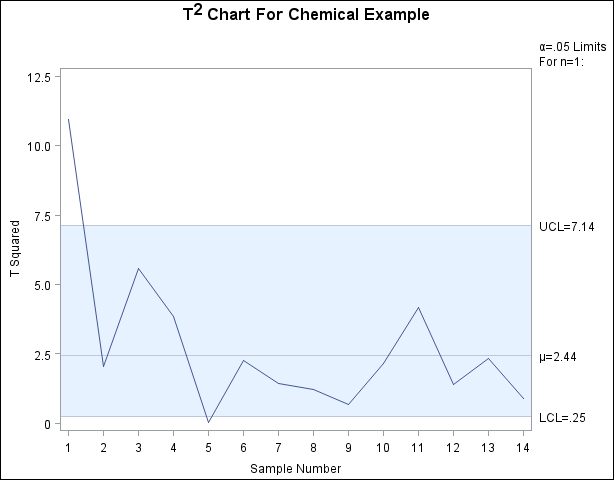
You can now use the data set Prin as input to the SHEWHART procedure to create the multivariate control chart displayed in Figure 15.223.
title 'T' m=(+0,+0.5) '2'
          m=(+0,-0.5) ' Chart For Chemical Example';
proc shewhart table=Prin;
   xchart tsquare*Sample /
      xsymbol  = mu
      nolegend ;
run;
The methods used in this example easily generalize to other types of multivariate control charts. You can create charts using the  and
and  distributions by using the appropriate CINV or FINV function in place of the BETAINV function. For details, refer to Alt (1985), Jackson (1980, 1991), and Ryan (1989).