Diagnosing and Modeling Autocorrelation
You can diagnose autocorrelation with an autocorrelation plot created with the ARIMA procedure.
ods graphics on;
ods select ChiSqAuto SeriesACFPlot SeriesPACFPlot;
proc arima data=Chemical plots(only)=series(acf pacf);
   identify var = xt;
run;
quit;
Refer to SAS/ETS User's Guide for details on the ARIMA procedure. The output, shown in Figure 15.193 and Figure 15.194, indicates that the data are highly autocorrelated with a lag 1 autocorrelation of 0.83.
Figure 15.193
Autocorrelation Check for Chemical Data
| Individual Measurements Chart |
The ARIMA Procedure
| Autocorrelation Check for White Noise | |||||||||
|---|---|---|---|---|---|---|---|---|---|
| To Lag | Chi-Square | DF | Pr > ChiSq | Autocorrelations | |||||
| 6 | 228.15 | 6 | <.0001 | 0.830 | 0.718 | 0.619 | 0.512 | 0.426 | 0.381 |
| 12 | 315.34 | 12 | <.0001 | 0.360 | 0.364 | 0.380 | 0.347 | 0.348 | 0.354 |
| 18 | 406.76 | 18 | <.0001 | 0.349 | 0.371 | 0.348 | 0.353 | 0.368 | 0.341 |
| 24 | 442.15 | 24 | <.0001 | 0.303 | 0.261 | 0.230 | 0.184 | 0.141 | 0.098 |
Figure 15.194
Autocorrelation Plots for Chemical Data
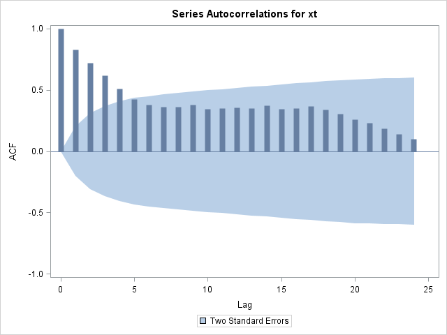
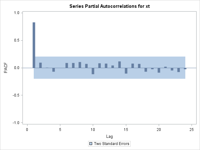
The partial autocorrelation plot in Figure 15.194 suggests that the data can be modeled with a first-order autoregressive model, commonly referred to as an AR(1) model.
 |
You can fit this model with the ARIMA procedure. The results in Figure 15.195 show that the equation of the fitted model is  .
.
ods select ParameterEstimates;
proc arima data=Chemical;
   identify var=xt;
   estimate p=1 method=ml;
run;
Figure 15.195
Fitted AR(1) Model
| Individual Measurements Chart |
The ARIMA Procedure
| Maximum Likelihood Estimation | |||||
|---|---|---|---|---|---|
| Parameter | Estimate | Standard Error | t Value | Approx Pr > |t| |
Lag |
| MU | 85.28375 | 2.32973 | 36.61 | <.0001 | 0 |
| AR1,1 | 0.84694 | 0.05221 | 16.22 | <.0001 | 1 |