Example 12.9 Optimal Design in the Presence of Covariance

[See OPTEX10 in the SAS/QC Sample Library]The BLOCKS statement finds a design that maximizes the determinant of the treatment information matrix, where depends on the block or covariate model. Alternatively, you can directly specify the matrix to find the D-optimal design when is the variance-covariance matrix for the runs. You can specify the data set containing the covariance matrix with the COVAR= option in the BLOCKS statement, listing the variables corresponding to the columns of the covariance matrix in the VAR= option. If you specify variables in the VAR= option, the values of these variables in the first observations in the data set will be used to define .

For example, suppose you want to compare the effects of seven different fertilizers on crop yield, by using seven long, narrow blocks of four plots each, as depicted in Figure 12.6.

In this case, it is reasonable to conjecture that closer plots within each block are more correlated. In particular, suppose that the plots are autocorrelated, so that the correlation matrix for the four plots in each block is of the form

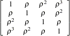where . If there is also an overall fixed effect due to blocks, the information matrix for the effect of fertilizer has the form , where

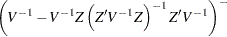In this formula, is the block diagonal matrix of the plot-by-plot correlation structure, with seven copies of on the diagonal. The matrix is the design matrix corresponding to the block effect. The optimal design should take into account this neighbor covariance structure as well as the block structure.

The following code uses the SAS/IML matrix language to construct by using and saves it in a data set named a:

proc iml;
   Blocks = int(((1:28)`-1)/4) + 1;      
   z = j(28,1) || designf(Blocks);      
   r = toeplitz(0.1**(0:3));            
   v = r;                               
   do i = 2 to 7; v = block(v,r); end;
   iv = inv(v);                         
   a = ginv(iv-iv*z*inv(z`*iv*z)*z`*iv); 
   create A from a;                     
   append from a;
quit;

Note that the data set is created with variables named COL1, COL2 ..., COL28, by default.

To find an allocation of fertilizers to plots that is optimal for detecting the fertilizer effect in the presence of this autocorrelation, simply specify a one-way model for the treatment effects and specify the data set A as the covariance matrix for the runs with the COVAR= option in the BLOCKS statement, as follows:

data Fertilizer; do f = 1 to 7; output; end;
proc optex data=Fertilizer seed=56672 coding=orth;
   class f;                            
   model f;                             
   blocks covar=A var=(COL1-COL28);                                   
   output out=NBD;
run;

The SAS/IML matrix language also provides a convenient way of listing the design.

proc iml;
   use NBD;                              
   read all var {f};                       
   NBD = shape(f,7,4);                  
   print NBD [format=2.];                  

These IML statements read in the selected levels of fertilizer and the reshape them into seven 4-run blocks before printing them. The resulting design is shown in Output 12.9.1. Note that it is not only a balanced incomplete block design, but it is also balanced for first neighbors; that is, every pair of treatments occur equally often on horizontally adjacent plots.

Output 12.9.1 Neighbor-Balanced BIBD for , , Found by Optimal Blocking

NBD
7	2	1	5
6	1	7	3
4	7	6	2
1	4	6	5
6	3	5	2
1	3	2	4
7	5	4	3