OUTPUT Statement: CAPABILITY Procedure

Example 5.18 Approximate Confidence Limits for Cpk

[See CPKCON3 in the SAS/QC Sample Library]This example illustrates how you can use the OUTPUT statement to compute confidence limits for the capability index $\text{[math]}$ .

You can request the approximate confidence limits given by Bissell (1990) with the keywords CPKLCL and CPKUCL in the OUTPUT statement. However, this is not the only method that has been proposed for computing confidence limits for $\text{[math]}$ . Zhang, Stenback, and Wardrop (1990), referred to here as ZSW, proposed approximate confidence limits of the form

$\text{[math]}$

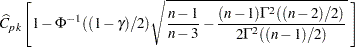
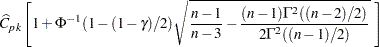
where $\text{[math]}$ is an estimator of the standard deviation of $\text{[math]}$ . Equation (8) of ZSW provides an approximation to the variance of $\text{[math]}$ from which one can obtain 100 $\text{[math]}$ % confidence limits for $\text{[math]}$ as

	$\text{[math]}$	$\text{[math]}$	$\text{[math]}$
	$\text{[math]}$	$\text{[math]}$	$\text{[math]}$

This assumes that $\text{[math]}$ is normally distributed. You can also compute approximate confidence limits based on equation (6) of ZSW, which provides an exact expression for the variance of $\text{[math]}$ .

The following program uses the methods of Bissell (1990) and ZSW to compute approximate confidence limits for $\text{[math]}$ for the variable Hardness in the data set Titanium (see Example 5.17).

proc capability data=Titanium noprint;
   var Hardness;
   specs lsl=0.8 usl=2.4;
   output out=Summary
       n    = n
       mean = mean
       std  = std
       lsl  = lsl
       usl  = usl
       cpk  = cpk
       cpklcl = cpklcl
       cpkucl = cpkucl
       cpl  = cpl
       cpu  = cpu ;

data Summary;
   set Summary;
   length Method $ 16;

   Method = "Bissell";
   lcl = cpklcl;
   ucl = cpkucl;
   output;

   * Assign confidence level;
   level = 0.95;
   aux   = probit( 1 - (1-level)/2 );

   Method = "ZSW Equation 6";
   zsw = log(0.5*n-0.5)
         + ( 2*(lgamma(0.5*n-1)-lgamma(0.5*n-0.5)) );
   zsw = sqrt((n-1)/(n-3)-exp(zsw));
   lcl = cpk*(1-aux*zsw);
   ucl = cpk*(1+aux*zsw);
   output;

   Method = "ZSW Equation 8";
   ds = 3*(cpu+cpl)/2;
   ms = 3*(cpl-cpu)/2;
   f1 = (1/3)*sqrt((n-1)/2)*gamma((n-2)/2)*(1/gamma((n-1)/2));
   f2 = sqrt(2/n)*(1/gamma(0.5))*exp(-n*0.5*ms*ms);
   f3 = ms*(1-(2*probnorm(-sqrt(n)*ms)));
   ex = f1*(ds-f2-f3);
   sd = ((n-1)/(9*(n-3)))*(ds**2-(2*ds*(f2+f3))+ms**2+(1/n));
   sd = sd-(ex*ex);
   sd = sqrt(sd);
   lcl = cpk-aux*sd;
   ucl = cpk+aux*sd;
   output;
run;

title "Approximate 95% Confidence Limits for Cpk";
proc print data = Summary noobs;
   var Method lcl cpk ucl;
run;

The results are shown in Output 5.18.1.

Output 5.18.1 Approximate Confidence Limits for $\text{[math]}$

Approximate 95% Confidence Limits for Cpk

Method	lcl	cpk	ucl
Bissell	1.43845	1.80818	2.17790
ZSW Equation 6	1.43596	1.80818	2.18040
ZSW Equation 8	1.42419	1.80818	2.19217

Note that there is fairly close agreement in the three methods.

You can display the confidence limits computed using Bissell’s approach on plots produced by the CAPABILITY procedure by specifying the keywords CPKLCL and CPKUCL in the INSET statement.

The following statements also compute an estimate of the index $\text{[math]}$ along with approximate limits by using the SPECIALINDICES option:

proc capability data=Titanium specialindices;
   var Hardness;
   specs lsl=0.8 usl=2.4;
run;

Output 5.18.2 Approximate Confidence Limits for $\text{[math]}$ using the SPECIALINDICES option

Approximate 95% Confidence Limits for Cpk

The CAPABILITY Procedure

Variable: Hardness (Hardness Measurement)

Process Capability Indices
Index	Value	95% Confidence Limits
Cp	2.005745	1.609575	2.401129
CPL	1.808179	1.438675	2.175864
CPU	2.203311	1.757916	2.646912
Cpk	1.808179	1.438454	2.177904