PROC SHEWHART: Constructing Charts for Numbers of Nonconformities (c Charts)

The SHEWHART Procedure

Constructing Charts for Numbers of Nonconformities (c Charts)

The following notation is used in this section:

$\text{[math]}$

expected number of nonconformities per unit produced by the process

$\text{[math]}$

number of nonconformities per unit in the $\text{[math]}$ th subgroup

$\text{[math]}$

total number of nonconformities in the $\text{[math]}$ th subgroup

$\text{[math]}$

number of inspection units in the $\text{[math]}$ th subgroup. Typically, $\text{[math]}$ and $\text{[math]}$ for $\text{[math]}$ charts. In general, $\text{[math]}$ .

$\text{[math]}$

average number of nonconformities per unit taken across subgroups. The quantity $\text{[math]}$ is computed as a weighted average:

$\text{[math]}$

number of subgroups

$\text{[math]}$

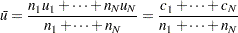
has a central $\text{[math]}$ distribution with $\text{[math]}$ degrees of freedom

Plotted Points

Each point on a $\text{[math]}$ chart represents the total number of nonconformities ( $\text{[math]}$ ) in a subgroup. For example, Figure 13.7.13 displays three sections of pipeline that are inspected for defective welds (indicated by an X). Each section represents a subgroup composed of a number of inspection units, which are 1000-foot-long sections. The number of units in the $\text{[math]}$ th subgroup is denoted by $\text{[math]}$ , which is the subgroup sample size. The value of $\text{[math]}$ can be fractional; Figure 13.7.13 shows $\text{[math]}$ units in the third subgroup.

Output 13.7.13 Terminology for $\text{[math]}$ Charts and $\text{[math]}$ Charts

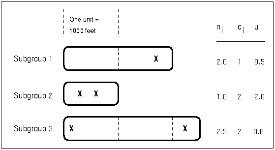
The number of nonconformities in the $\text{[math]}$ th subgroup is denoted by $\text{[math]}$ . The number of nonconformities per unit in the $\text{[math]}$ th subgroup is denoted by $\text{[math]}$ . In Figure 13.7.13, the number of welds per inspection unit in the third subgroup is $\text{[math]}$ .

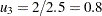A $\text{[math]}$ chart created with the UCHART statement plots the quantity $\text{[math]}$ for the $\text{[math]}$ th subgroup (see UCHART Statement). An advantage of a $\text{[math]}$ chart is that the value of the central line at the $\text{[math]}$ th subgroup does not depend on $\text{[math]}$ . This is not the case for a $\text{[math]}$ chart, and consequently, a $\text{[math]}$ chart is often preferred when the number of units $\text{[math]}$ is not constant across subgroups.

Central Line

On a $\text{[math]}$ chart, the central line indicates an estimate for $\text{[math]}$ , which is computed as $\text{[math]}$ . If you specify a known value ( $\text{[math]}$ ) for $\text{[math]}$ , the central line indicates the value of $\text{[math]}$ .

Note that the central line varies with subgroup sample size $\text{[math]}$ . When $\text{[math]}$ for all subgroups, the central line has the constant value $\text{[math]}$ .

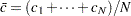Control Limits

You can compute the limits in the following ways:

as a specified multiple ( $\text{[math]}$ ) of the standard error of $\text{[math]}$ above and below the central line. The default limits are computed with $\text{[math]}$ (these are referred to as $\text{[math]}$ limits).
as probability limits defined in terms of $\text{[math]}$ , a specified probability that $\text{[math]}$ exceeds the limits

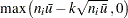
The lower and upper control limits, LCLC and UCLC respectively, are given by

	$\text{[math]}$	$\text{[math]}$	$\text{[math]}$
	$\text{[math]}$	$\text{[math]}$	$\text{[math]}$

The upper and lower control limits vary with the number of inspection units per subgroup $\text{[math]}$ . If $\text{[math]}$ for all subgroups, the control limits have constant values.

	$\text{[math]}$	$\text{[math]}$	$\text{[math]}$
	$\text{[math]}$	$\text{[math]}$	$\text{[math]}$

An upper probability limit UCLC for $\text{[math]}$ can be determined using the fact that

$\text{[math]}$

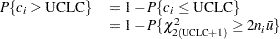The upper probability limit UCLC is then calculated by setting

$\text{[math]}$

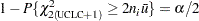and solving for UCLC.

A similar approach is used to calculate the lower probability limit LCLC, using the fact that

$\text{[math]}$

The lower probability limit LCLC is then calculated by setting

$\text{[math]}$

and solving for LCLC. This assumes that the process is in statistical control and that $\text{[math]}$ has a Poisson distribution. For more information, refer to Johnson, Kotz, and Kemp (1992). Note that the probability limits vary with the number of inspection units per subgroup ( $\text{[math]}$ ) and are asymmetric about the central line.

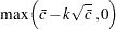
If a standard value $\text{[math]}$ is available for $\text{[math]}$ , replace $\text{[math]}$ with $\text{[math]}$ in the formulas for the control limits. You can specify parameters for the limits as follows:

Specify $\text{[math]}$ with the SIGMAS= option or with the variable _SIGMAS_ in a LIMITS= data set.
Specify $\text{[math]}$ with the ALPHA= option or with the variable _ALPHA_ in a LIMITS= data set.
Specify a constant nominal sample size $\text{[math]}$ for the control limits with the LIMITN= option or with the variable _LIMITN_ in a LIMITS= data set.
Specify $\text{[math]}$ with the U0= option or with the variable _U_ in a LIMITS= data set.

Top of Page