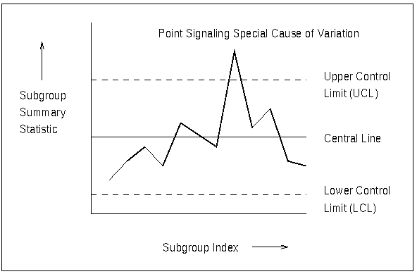
Figure 13.1 illustrates a typical Shewhart chart.

Figure 13.1 A Shewhart Control Chart

All Shewhart charts have the following characteristics:

• Each point represents a summary statistic computed from a sample of measurements of a quality characteristic. For example, the summary statistic might be the average value of a critical dimension of five items selected at random, or it might be the proportion of nonconforming items in a sample of 100 items.

• The vertical axis of a Shewhart chart is scaled in the same units as the summary statistic.

• The samples from which the summary statistics are computed are referred to as rational subgroups or subgroup samples. The organization of the data into subgroups is critical to the interpretation of a Shewhart chart. Shewhart (1931) advocated selecting rational subgroups so that variation within subgroups is minimized and variation among subgroups is maximized; this makes the chart more sensitive to shifts in the process level. Various approaches to subgrouping are discussed by Grant and Leavenworth (1988), Montgomery (1996), and Kume (1985).

• The horizontal axis of a Shewhart chart identifies the subgroup samples. Frequently, the samples are indexed according to the order in which they were taken or the time at which they were taken. Subgroup samples can also be assigned labels that indicate some other type of classification (for example, lot number).

• The central line on a Shewhart chart indicates the average (expected value) of the summary statistic when the process is in statistical control.

• The upper and lower control limits, labeled UCL and LCL, respectively, indicate the range of variation to be expected in the summary statistic when the process is in statistical control. The control limits are commonly computed as 3 limits¹ representing three standard errors² of variation in the summary statistic above and below the central line. However, the limits can also be determined using a multiple of the standard error other than three, or from a specified probability () that a single summary statistic will exceed the limits when the process is in statistical control. Limits determined by the latter method are referred to as probability limits.

  The control limits are also determined by the subgroup sample size because the standard error of the summary statistic is a function of sample size. If the sample size is constant across subgroups, the control limits are typically horizontal lines, as in Figure 13.1. However, if the sample size varies from subgroup to subgroup, the limits are usually adjusted to compensate for the effect of sample size, resulting in step-like boundaries.

  Control limits can be estimated from the data being analyzed, or they can be standard, previously determined values. Estimated limits are often used when statistical control is being established, and standard limits are often used when statistical control is being maintained.

• A point outside the control limits signals the presence of a special cause of variation. Additionally, tests for special causes (also referred to as Western Electric rules and runs tests) can signal an out-of-control condition if a statistically unusual pattern of points is observed in the control chart. For example, one pattern used to diagnose the existence of a trend is seven consecutive steadily increasing points.

  When the process is in statistical control, a point may fall outside the control limits purely by chance, resulting in a false out-of-control signal. However, when the Shewhart chart correctly signals the presence of a special cause, additional action is needed to determine the nature of the problem and eliminate it.