| The MACONTROL Procedure |
Constructing EWMA Charts
The following notation is used in this section:
|
exponentially weighted moving average for the |
|
EWMA weight parameter |
|
process mean (expected value of the population of measurements) |
|
process standard deviation (standard deviation of the population of measurements) |
|
|
|
sample size of |
|
mean of measurements in |
|
weighted average of subgroup means |
|
inverse standard normal function |


 th measurement in
 , then the subgroup mean reduces to the single observation in the subgroup
Plotted Points
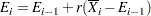
Each point on the chart indicates the value of the exponentially weighted moving average (EWMA) for that subgroup. The EWMA for the  th subgroup (
 ) is defined recursively as
 |
where  is a weight parameter
  . Some authors (for example, Hunter 1986 and Crowder 1987a,b) use the symbol
  instead of for the weight. You can specify the weight with the WEIGHT= option in the EWMACHART statement or with the variable _WEIGHT_ in a LIMITS= data set. If you specify a known value (
 ) for
) for  ,
,  ; otherwise,
  .
.
The preceding equation can be rewritten as
 |
which expresses the current EWMA as the previous EWMA plus the weighted error in the prediction of the current mean based on the previous EWMA.
The EWMA for the th subgroup can also be written as
 |
which expresses the EWMA as a weighted average of past subgroup means, where the weights decline exponentially, and the heaviest weight is assigned to the most recent subgroup mean.
Central Line
By default, the central line on an EWMA chart indicates an estimate for , which is computed as
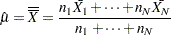 |
If you specify a known value () for , the central line indicates the value of .
Control Limits
You can compute the limits in the following ways:
as a specified multiple (
 ) of the standard error of above and below the central line. The default limits are computed with
  (these are referred to as
  limits).
 as probability limits defined in terms of
 , a specified probability that exceeds the limits
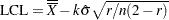
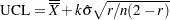
The following table presents the formulas for the limits:
Control Limits |
|---|
LCL = lower limit = |
UCL = upper limit = |
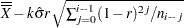
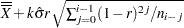
Probability Limits |
|---|
LCL = lower limit = |
UCL = upper limit = |
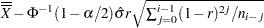
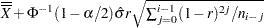
These formulas assume that the data are normally distributed. If standard values and  are available for and
  , respectively, replace
  with and
  with in Table 9.3. Note that the limits vary with both
  and .
and .
If the subgroup sample sizes are constant ( ), the formulas for the control limits simplify to
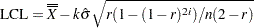 |
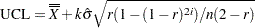 |
Consequently, when the subgroup sample sizes are constant, the width of the control limits increases monotonically with . For probability limits, replace with  in the previous equations. Refer to Roberts (1959) and Montgomery (1996).
As becomes large, the upper and lower control limits approach constant values:
 |
 |
Some authors base the control limits for EWMA charts on the asymptotic expressions in the two previous equations. For asymptotic probability limits, replace with in these equations. You can display asymptotic limits by specifying the ASYMPTOTIC option.
Uniformly weighted moving average charts and exponentially weighted moving average charts have similar properties, and their asymptotic control limits are identical provided that
 |
where  is the weight factor for uniformly weighted moving average charts. Refer to Wadsworth, Stephens, and Godfrey (1986) and the American Society for Quality Control (1983).
You can specify parameters for the EWMA limits as follows:
Specify
with the SIGMAS= option or with the variable _SIGMAS_ in a LIMITS= data set. Specify
with the ALPHA= option or with the variable _ALPHA_ in a LIMITS= data set. Specify a constant nominal sample size
 for the control limits with the LIMITN= option or with the variable _LIMITN_ in a LIMITS= data set.
 Specify
with the WEIGHT= option or with the variable _WEIGHT_ in a LIMITS= data set. Specify
with the MU0= option or with the variable _MEAN_ in a LIMITS= data set. Specify
with the SIGMA0= option or with the variable _STDDEV_ in a LIMITS= data set.
Choosing the Value of the Weight Parameter
Various approaches have been proposed for choosing the value of .
Hunter (1986) states that the choice "can be left to the judgment of the quality control analyst" and points out that the smaller the value of
, "the greater the influence of the historical data." Hunter (1986) also discusses a least squares procedure for estimating
from the data, assuming an exponentially weighted moving average model for the data. In this context, the fitted EWMA model provides a forecast of the process that is the basis for dynamic process control. You can use the ARIMA procedure in SAS/ETS® software to compute the least squares estimate of . (Refer to SAS/ETS 9.22 User's Guide for information about PROC ARIMA.) Also see Autocorrelation in Process Data. A number of authors have studied the design of EWMA control schemes based on average run length (ARL) computations. The ARL is the expected number of points plotted before a shift is detected. Ideally, the ARL should be short when a shift occurs, and it should be long when there is no shift (the process is in control.) The effect of
on the ARL was described by Roberts (1959), who used simulation methods. The ARL function was approximated and tabulated by Robinson and Ho (1978), and a more general method for studying run-length distributions of EWMA charts was given by Crowder (1987a, 1987b). Unlike Hunter (1986), these authors assume the data are independent and identically distributed; typically the normal distribution is assumed for the data, although the methods extend to nonnormal distributions. A more detailed discussion of the ARL approach follows.
Average run lengths for two-sided EWMA charts are shown in Table 9.4, which is patterned after Table 1 of Crowder (1987a, 1987b). The ARLs were computed using the EWMAARL DATA step function (see EWMAARL Function for details on the EWMAARL function). Note that Crowder (1987a, 1987b). uses the notation L in place of and the notation in place of .
You can use Table 9.4 to find a combination of and that yields a desired ARL for an in-control process ( ) and for a specified shift of
  . Note that is assumed to be standardized; in other words, if a shift of
  is to be detected in the process mean , and if is the process standard deviation, you should select the table entry with
 |
where  is the subgroup sample size. Thus, can be regarded as the shift in the sampling distribution of the subgroup mean.
For example, suppose you want to construct an EWMA scheme with an in-control ARL of 90 and an ARL of 9 for detecting a shift of  . Table 9.4 shows that the combination
  and
and  yields an in-control ARL of 91.17 and an ARL of 8.27 for .
Crowder (1987a, 1987b) cautions that setting the in-control ARL at a desired level does not guarantee that the probability of an early false signal is acceptable. For further details concerning the distribution of the ARL, refer to Crowder (1987a, 1987b).
In addition to using Table 9.4 or the EWMAARL DATA step function to choose a EWMA scheme with desired average run length properties, you can use them to evaluate an existing EWMA scheme. For example, the "Getting Started" section of this chapter contains EWMA schemes with  and . The following statements use the EWMAARL function to compute the in-control ARL and the ARLs for shifts of
  and
and  :
:
data arlewma;
   arlin = ewmaarl(  0,0.3,3.0);
   arl1  = ewmaarl(.25,0.3,3.0);
   arl2  = ewmaarl(.50,0.3,3.0);
run;
The in-control ARL is 465.553, the ARL for  is 178.741, and the ARL for
  is 53.1603. See Example 9.5 for an illustration of how to use the EWMAARL function to compute average run lengths for various EWMA schemes and shifts.
|
|||||||
|---|---|---|---|---|---|---|---|
|
|
0.05 |
0.10 |
0.25 |
0.50 |
0.75 |
1.00 |
2.0 |
0.00 |
127.53 |
73.28 |
38.56 |
26.45 |
22.88 |
21.98 |
2.0 |
0.25 |
43.94 |
34.49 |
24.83 |
20.12 |
18.86 |
19.13 |
2.0 |
0.50 |
18.97 |
15.53 |
12.74 |
11.89 |
12.34 |
13.70 |
2.0 |
0.75 |
11.64 |
9.36 |
7.62 |
7.29 |
7.86 |
9.21 |
2.0 |
1.00 |
8.38 |
6.62 |
5.24 |
4.91 |
5.26 |
6.25 |
2.0 |
1.25 |
6.56 |
5.13 |
3.96 |
3.59 |
3.76 |
4.40 |
2.0 |
1.50 |
5.41 |
4.20 |
3.19 |
2.80 |
2.84 |
3.24 |
2.0 |
1.75 |
4.62 |
3.57 |
2.68 |
2.29 |
2.26 |
2.49 |
2.0 |
2.00 |
4.04 |
3.12 |
2.32 |
1.95 |
1.88 |
2.00 |
2.0 |
2.25 |
3.61 |
2.78 |
2.06 |
1.70 |
1.61 |
1.67 |
2.0 |
2.50 |
3.26 |
2.52 |
1.85 |
1.51 |
1.42 |
1.45 |
2.0 |
2.75 |
2.99 |
2.32 |
1.69 |
1.37 |
1.29 |
1.29 |
2.0 |
3.00 |
2.76 |
2.16 |
1.55 |
1.26 |
1.19 |
1.19 |
2.0 |
3.25 |
2.56 |
2.03 |
1.43 |
1.18 |
1.13 |
1.12 |
2.0 |
3.50 |
2.39 |
1.93 |
1.32 |
1.12 |
1.08 |
1.07 |
2.0 |
3.75 |
2.26 |
1.83 |
1.24 |
1.08 |
1.05 |
1.04 |
2.0 |
4.00 |
2.15 |
1.73 |
1.17 |
1.05 |
1.03 |
1.02 |
2.5 |
0.00 |
379.09 |
223.35 |
124.18 |
91.17 |
82.49 |
80.52 |
2.5 |
0.25 |
73.98 |
66.59 |
59.66 |
58.33 |
61.07 |
65.77 |
2.5 |
0.50 |
26.63 |
23.63 |
23.28 |
27.16 |
33.26 |
41.49 |
2.5 |
0.75 |
15.41 |
12.95 |
11.96 |
13.96 |
18.05 |
24.61 |
2.5 |
1.00 |
10.79 |
8.75 |
7.52 |
8.27 |
10.57 |
14.92 |
2.5 |
1.25 |
8.31 |
6.60 |
5.39 |
5.52 |
6.75 |
9.46 |
2.5 |
1.50 |
6.78 |
5.31 |
4.18 |
4.03 |
4.65 |
6.30 |
2.5 |
1.75 |
5.75 |
4.46 |
3.43 |
3.14 |
3.43 |
4.41 |
2.5 |
2.00 |
5.00 |
3.86 |
2.92 |
2.57 |
2.67 |
3.24 |
2.5 |
2.25 |
4.43 |
3.42 |
2.56 |
2.18 |
2.17 |
2.49 |
2.5 |
2.50 |
4.00 |
3.07 |
2.29 |
1.90 |
1.83 |
2.00 |
2.5 |
2.75 |
3.64 |
2.80 |
2.08 |
1.69 |
1.59 |
1.67 |
2.5 |
3.00 |
3.36 |
2.57 |
1.91 |
1.52 |
1.41 |
1.45 |
2.5 |
3.25 |
3.12 |
2.39 |
1.77 |
1.39 |
1.29 |
1.29 |
2.5 |
3.50 |
2.92 |
2.24 |
1.64 |
1.28 |
1.19 |
1.19 |
2.5 |
3.75 |
2.74 |
2.13 |
1.52 |
1.20 |
1.13 |
1.12 |
2.5 |
4.00 |
2.58 |
2.04 |
1.42 |
1.13 |
1.08 |
1.07 |
3.0 |
0.00 |
1383.62 |
842.15 |
502.90 |
397.46 |
374.50 |
370.40 |
3.0 |
0.25 |
133.61 |
144.74 |
171.09 |
208.54 |
245.76 |
281.15 |
3.0 |
0.50 |
37.33 |
37.41 |
48.45 |
75.35 |
110.95 |
155.22 |
3.0 |
0.75 |
19.95 |
17.90 |
20.16 |
31.46 |
50.92 |
81.22 |
3.0 |
1.00 |
13.52 |
11.38 |
11.15 |
15.74 |
25.64 |
43.89 |
3.0 |
1.25 |
10.24 |
8.32 |
7.39 |
9.21 |
14.26 |
24.96 |
3.0 |
1.50 |
8.26 |
6.57 |
5.47 |
6.11 |
8.72 |
14.97 |
3.0 |
1.75 |
6.94 |
5.45 |
4.34 |
4.45 |
5.80 |
9.47 |
3.0 |
2.00 |
6.00 |
4.67 |
3.62 |
3.47 |
4.15 |
6.30 |
3.0 |
2.25 |
5.30 |
4.10 |
3.11 |
2.84 |
3.16 |
4.41 |
3.0 |
2.50 |
4.76 |
3.67 |
2.75 |
2.41 |
2.52 |
3.24 |
3.0 |
2.75 |
4.32 |
3.32 |
2.47 |
2.10 |
2.09 |
2.49 |
3.0 |
3.00 |
3.97 |
3.05 |
2.26 |
1.87 |
1.79 |
2.00 |
3.0 |
3.25 |
3.67 |
2.82 |
2.09 |
1.69 |
1.57 |
1.67 |
3.0 |
3.50 |
3.42 |
2.62 |
1.95 |
1.53 |
1.41 |
1.45 |
3.0 |
3.75 |
3.22 |
2.45 |
1.84 |
1.41 |
1.29 |
1.29 |
3.0 |
4.00 |
3.04 |
2.30 |
1.73 |
1.31 |
1.20 |
1.19 |
3.5 |
0.00 |
12851.0 |
4106.4 |
2640.16 |
2227.34 |
2157.99 |
2149.34 |
3.5 |
0.25 |
281.09 |
381.29 |
625.78 |
951.18 |
1245.90 |
1502.76 |
3.5 |
0.50 |
53.58 |
64.72 |
123.43 |
267.36 |
468.68 |
723.81 |
3.5 |
0.75 |
25.62 |
25.33 |
38.68 |
88.70 |
182.12 |
334.40 |
3.5 |
1.00 |
16.65 |
14.79 |
17.71 |
35.97 |
78.05 |
160.95 |
3.5 |
1.25 |
12.36 |
10.37 |
10.48 |
17.64 |
37.15 |
81.80 |
3.5 |
1.50 |
9.86 |
8.00 |
7.25 |
10.19 |
19.63 |
43.96 |
3.5 |
1.75 |
8.22 |
6.54 |
5.52 |
6.70 |
11.46 |
24.96 |
3.5 |
2.00 |
7.07 |
5.55 |
4.47 |
4.86 |
7.33 |
14.97 |
3.5 |
2.25 |
6.21 |
4.83 |
3.77 |
3.78 |
5.08 |
9.47 |
3.5 |
2.50 |
5.55 |
4.29 |
3.28 |
3.10 |
3.76 |
6.30 |
3.5 |
2.75 |
5.03 |
3.87 |
2.91 |
2.63 |
2.94 |
4.41 |
3.5 |
3.00 |
4.60 |
3.54 |
2.63 |
2.30 |
2.40 |
3.24 |
3.5 |
3.25 |
4.25 |
3.26 |
2.41 |
2.05 |
2.03 |
2.49 |
3.5 |
3.50 |
3.95 |
3.03 |
2.23 |
1.85 |
1.76 |
2.00 |
3.5 |
3.75 |
3.70 |
2.84 |
2.10 |
1.69 |
1.56 |
1.67 |
3.5 |
4.00 |
3.47 |
2.66 |
1.99 |
1.55 |
1.40 |
1.45 |
Copyright © SAS Institute, Inc. All Rights Reserved.