The FREQ Procedure

Odds Ratio and Relative Risks for 2  2 Tables
Odds Ratio
The odds ratio is a useful measure of association for a variety of study designs. For a retrospective design called a case-control study, the odds ratio can be used to estimate the relative risk when the probability of positive response is small (Agresti 2002). In a case-control study, two independent samples are identified based on a binary (yes-no) response variable, and the conditional distribution of a binary explanatory variable is examined within fixed levels of the response variable. For more information, see Stokes, Davis, and Koch (2012), Agresti (2013), and Agresti (2007).
The odds of a positive response (column 1) in row 1 is  . Similarly, the odds of a positive response in row 2 is
  . The odds ratio is formed as the ratio of the row 1 odds to the row 2 odds. The odds ratio for a
  table is defined as
![\[ \mathit{OR} = \frac{n_{11}/n_{12}}{n_{21}/n_{22}} = \frac{n_{11} ~ n_{22}}{n_{12} ~ n_{21}} \]](images/procstat_freq0399.png)
The odds ratio can be any nonnegative number. When the row and column variables are independent, the true value of the odds ratio is 1. An odds ratio greater than 1 indicates that the odds of a positive response are higher in row 1 than in row 2. An odds ratio less than 1 indicates that the odds of a positive response are higher in row 2. The strength of association increases as the deviation from 1 increases.
The transformation 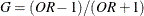 transforms the odds ratio to the range (–1,1), where G = 0 when
  ; G = –1 when
  ; and G approaches 1 as OR approaches infinity. G is the gamma statistic, which PROC FREQ computes when you specify the MEASURES option.
Confidence Limits for the Odds Ratio
The following types of confidence limits are available for the odds ratio: exact, exact mid-p, likelihood ratio, score, Wald, and Wald modified.
Wald Confidence Limits
The asymptotic Wald confidence limits are based on a log transformation of the odds ratio (Woolf 1955; Haldane 1955). PROC FREQ computes the Wald confidence limits as
![\[ \left( ~ \mathit{OR} \times \exp ( -z \sqrt {v} ), ~ ~ \mathit{OR} \times \exp ( z \sqrt {v} ) ~ \right) \]](images/procstat_freq0403.png)
where
![\[ v = \mr{Var} (\ln \mathit{OR}) = 1/n_{11} + 1/n_{12} + 1/n_{21} + 1/n_{22} \]](images/procstat_freq0404.png)
and z is the  th percentile of the standard normal distribution. The confidence level
  is determined by the ALPHA=
option in the TABLES statement; by default, ALPHA=0.05, which produces 95% confidence limits for the odds ratio. If any of
the four cell frequencies are 0, v is undefined and the Wald confidence limits cannot be computed. For more information, see Agresti (2013, p. 70).
is determined by the ALPHA=
option in the TABLES statement; by default, ALPHA=0.05, which produces 95% confidence limits for the odds ratio. If any of
the four cell frequencies are 0, v is undefined and the Wald confidence limits cannot be computed. For more information, see Agresti (2013, p. 70).
Wald Modified Confidence Limits
PROC FREQ computes Wald modified confidence limits (Haldane 1955) for the odds ratio by replacing the  by
by  in the estimator
  and the variance v as follows:
![\[ \mathit{OR} = \frac{(n_{11} + 0.5) ~ (n_{22} + 0.5)}{(n_{12} + 0.5) ~ (n_{21} + 0.5)} \]](images/procstat_freq0407.png)
![\[ v = \mr{Var} (\ln \mathit{OR}) = 1/(n_{11} + 0.5) + 1/(n_{12} + 0.5) + 1/(n_{21} + 0.5) + 1/(n_{22} + 0.5) \]](images/procstat_freq0408.png)
The modified confidence limits are then computed as
where z is the th percentile of the standard normal distribution. For more information, see Fleiss, Levin, and Paik (2003) and Agresti (2013).
Score Confidence Limits
Score confidence limits for the odds ratio (Miettinen and Nurminen 1985) are computed by inverting score tests for the odds ratio. A score-based chi-square test statistic for the null hypothesis
that the odds ratio equals  can be expressed as
![\[ Q(\theta ) = \{ n_{1 \cdot } \left( \hat{p}_1 - \tilde{p}_1 \right) \} ^2 ~ / ~ \{ n / (n-1) \} ~ \{ 1 / \left( n_{1 \cdot } \tilde{p}_1 ( 1 - \tilde{p}_1 ) \right) + 1 / \left( n_{2 \cdot } \tilde{p}_2 ( 1 - \tilde{p}_2 ) \right) \} ^{-1} \]](images/procstat_freq0410.png)
where  is the observed row 1 risk (
 ), and
  and
and  are the maximum likelihood estimates of the row 1 and row 2 risks under the restriction that the odds ratio (
 ) is . For more information, see Miettinen and Nurminen (1985) and Miettinen (1985, chapter 14).
The  % score confidence interval for the odds ratio consists of all values of for which the test statistic
  falls in the acceptance region,
![\[ \{ \theta : Q(\theta ) < \chi ^2_{1, \alpha } \} \]](images/procstat_freq0415.png)
where  is the 100
 th percentile of the chi-square distribution with 1 degree of freedom. For more information about score confidence limits,
see Agresti (2013).
th percentile of the chi-square distribution with 1 degree of freedom. For more information about score confidence limits,
see Agresti (2013).
By default, the score confidence limits include the bias correction factor  in the denominator of (Miettinen and Nurminen 1985, p. 217). If you specify the CL=SCORE(CORRECT=NO) option, PROC FREQ does not include this factor in the computation.
The maximum likelihood estimates of  and
and  , subject to the constraint that the odds ratio is , are computed as
![\[ \tilde{p}_2 = \left( -b + \sqrt { b^2 - 4 a c } \right) / 2a \hspace{.15in} \mr{and} \hspace{.15in} \tilde{p}_1 = \tilde{p}_2 \theta / \left( 1 + \tilde{p}_2 (\theta - 1) \right) \]](images/procstat_freq0416.png)
where
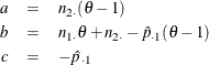
For more information, see Miettinen and Nurminen (1985, pp. 217–218) and Miettinen (1985, chapter 14).
Likelihood Ratio Confidence Limits
Likelihood ratio (profile likelihood) confidence limits for the odds ratio are computed by inverting likelihood ratio tests.
The likelihood ratio test statistic for the null hypothesis that the odds ratio equals can be expressed as
![\[ G^2(\theta ) ~ = ~ 2 ~ \bigl ( n_{11} \ln ( \hat{p}_1 / \tilde{p}_1 ) ~ + ~ n_{12} \ln ( (1-\hat{p}_1) / (1-\tilde{p}_1 ) ~ + ~ n_{21} \ln ( \hat{p}_2 / \tilde{p}_2 ) ~ + ~ n_{22} \ln ( (1-\hat{p}_2 / (1-\tilde{p}_2 ) \bigr ) \]](images/procstat_freq0418.png)
where  is the observed row i risk () and
  is the maximum likelihood estimate of the row i risk under the restriction that the odds ratio is . The computation of the maximum likelihood estimates is described in the subsection "Score Confidence Limits"
in this section. For more information, see Agresti (2013), Miettinen and Nurminen (1985), and Miettinen (1985, chapter 14).
is the maximum likelihood estimate of the row i risk under the restriction that the odds ratio is . The computation of the maximum likelihood estimates is described in the subsection "Score Confidence Limits"
in this section. For more information, see Agresti (2013), Miettinen and Nurminen (1985), and Miettinen (1985, chapter 14).
The % likelihood ratio confidence interval for the odds ratio consists of all values of for which the test statistic  falls in the acceptance region,
![\[ \{ \theta : G^2(\theta ) < \chi ^2_{1, \alpha } \} \]](images/procstat_freq0422.png)
where is the 100th percentile of the chi-square distribution with 1 degree of freedom.
Exact Confidence Limits
PROC FREQ computes exact confidence limits for the odds ratio by inverting two one-sided (equal-tail) exact tests that are
based on the noncentral hypergeometric distribution, where the distribution is conditional on the observed marginal totals
of the table. The exact confidence limits  and
and  are the solutions to the equations
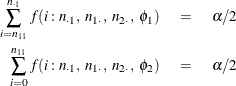
where
![\[ f( i : n_{\cdot 1}, ~ n_{1 \cdot }, ~ n_{2 \cdot }, ~ \phi ) = \binom {n_{1 \cdot }}{i} \binom {n_{2 \cdot }}{n_{\cdot 1} - i} ~ \phi ^ i ~ ~ / ~ ~ \sum _{i=0}^{n_{\cdot 1}} \binom {n_{1 \cdot }}{i} \binom {n_{2 \cdot }}{n_{\cdot 1}-i} ~ \phi ^ i \]](images/procstat_freq0426.png)
For more information, see Fleiss, Levin, and Paik (2003), Thomas (1971), and Gart (1971).
Because this is a discrete problem, the confidence coefficient for the exact confidence interval is not exactly but is at least ; thus, these confidence limits are conservative. For more information, see Agresti (1992).
When the odds ratio is 0, which occurs when either  or
or  , PROC FREQ sets the lower exact confidence limit to 0 and determines the upper limit by using the level (instead of
  ). Similarly, when the odds ratio is infinity, which occurs when either
  or
or  , PROC FREQ sets the upper exact confidence limit to infinity and determines the lower limit by using level .
Exact Mid-p Confidence Limits
PROC FREQ computes exact mid-p confidence limits for the odds ratio by inverting two one-sided hypergeometric tests that include mid-p tail areas. The mid-p approach replaces the probability of the observed table by half of that probability in the hypergeometric probability sums,
which are described in the subsection "Exact Confidence Limits"
in this section. The exact mid-p confidence limits and are the solutions to the equations
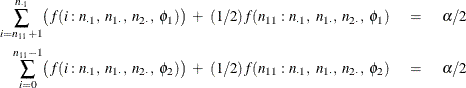
where
![\[ f( i : n_{\cdot 1}, n_{1 \cdot }, n_{2 \cdot }, \phi ) = \binom {n_{1 \cdot }}{i} \binom {n_{2 \cdot }}{n_{\cdot 1} - i} ~ \phi ^ i ~ ~ / ~ ~ \sum _{i=0}^{n_{\cdot 1}} \binom {n_{1 \cdot }}{i} \binom {n_{2 \cdot }}{n_{\cdot 1}-i} ~ \phi ^ i \]](images/procstat_freq0432.png)
For more information, see Agresti (2013).
When the odds ratio is 0, which occurs when either or , PROC FREQ sets the lower exact confidence limit to 0 and determines the upper limit by using the level (instead of ). Similarly, when the odds ratio is infinity, which occurs when either or , PROC FREQ sets the upper exact confidence limit to infinity and determines the lower limit by using level .
Relative Risks
Relative risks are useful measures in cohort (prospective) study designs, where two samples are identified based on the presence or absence of an explanatory factor. The two samples are observed in future time for the binary (yes-no) response variable under study. Relative risks are also useful in cross-sectional studies, where two variables are observed simultaneously. For more information, see Stokes, Davis, and Koch (2012) and Agresti (2007).
The relative risk is the ratio of the row 1 risk to the row 2 risk in a table. The column 1 risk in row 1 is the proportion of row 1 observations that are classified in column 1, which can be expressed
as
![\[ p_1 = n_{11} ~ / ~ n_{1 \cdot } \]](images/procstat_freq0433.png)
Similarly, the column 1 risk in row 2 is
![\[ p_2 = n_{21} ~ / ~ n_{2 \cdot } \]](images/procstat_freq0434.png)
The column 1 relative risk is computed as
![\[ R = p_1 ~ / ~ p_2 \]](images/procstat_freq0435.png)
A relative risk greater than 1 indicates that the probability of positive response is greater in row 1 than in row 2. Similarly, a relative risk less than 1 indicates that the probability of positive response is less in row 1 than in row 2. The strength of association increases as the deviation from 1 increases.
Confidence Limits for the Relative Risk
PROC FREQ provides the following types of confidence limits for the relative risk: exact unconditional, likelihood ratio, score, Wald, and Wald modified.
Wald Confidence Limits
The asymptotic Wald confidence limits are based on a log transformation of the relative risk. PROC FREQ computes the Wald
confidence limits for the column 1 relative risk as
![\[ \left( ~ \hat{r} \times \exp ( -z \sqrt {v} ) , ~ ~ \hat{r} \times \exp ( z \sqrt {v} ) ~ \right) \]](images/procstat_freq0436.png)
where  is the observed value of the relative risk,
  , and
, and
![\[ v = \mr{Var}(\ln (\hat{r})) = \bigl ( (1-\hat{p}_1) / n_{11} \bigr ) ~ + ~ \bigl ( (1-\hat{p}_2) / n_{21} \bigr ) \]](images/procstat_freq0439.png)
and z is the th percentile of the standard normal distribution. The confidence level is determined by the ALPHA=
option in the TABLES statement; by default, ALPHA=0.05, which produces 95% confidence limits. If either cell frequency  or
or  is 0, then v is undefined and the Wald confidence limits cannot be computed.
PROC FREQ computes the confidence limits for the column 2 relative risk in the same way.
Wald Modified Confidence Limits
PROC FREQ computes Wald modified confidence limits (Haldane 1955) for the relative risk by replacing the with and the  with
with  in the estimator R and the variance v as follows:
![\[ \hat{r}_\mi {m} = \hat{p}_1 / \hat{p}_2 = \frac{ (n_{11} + 0.5) / (n_{1 \cdot } + 0.5) }{ (n_{21} + 0.5) / (n_{2 \cdot } + 0.5) } \]](images/procstat_freq0442.png)
![\[ v = \mr{Var}(\ln (\hat{r}_\mi {m})) = 1/(n_{11} + 0.5) + 1/(n_{21} + 0.5) - 1/(n_{1 \cdot } + 0.5) - 1/(n_{2 \cdot } + 0.5) \]](images/procstat_freq0443.png)
The confidence limits are computed as
![\[ \left( ~ \hat{r}_\mi {m} \times \exp ( -z \sqrt {v} ), ~ ~ \hat{r}_ mi{m} \times \exp ( z \sqrt {v} ) ~ \right) \]](images/procstat_freq0444.png)
where z is the th percentile of the standard normal distribution. For more information, see Fleiss, Levin, and Paik (2003) and Agresti (2013).
Score Confidence Limits
Score confidence limits (Miettinen and Nurminen 1985; Farrington and Manning 1990) are computed by inverting score tests for the relative risk.
A score-based chi-square test statistic for the null hypothesis that the relative risk is  can be expressed as
![\[ Q(r_0) = ( \hat{p}_1 - r_0 \hat{p}_2 )^2 ~ / ~ \widetilde{\mr{Var}}(r_0) \]](images/procstat_freq0446.png)
where and  are the observed row 1 and row 2 risks (proportions), respectively,
![\[ \widetilde{\mr{Var}}(r_0) = \left( n / (n-1) \right) ~ \left( ~ \tilde{p}_1 (1-\tilde{p}_1) / n_{1 \cdot } ~ +~ {r_0}^2 ~ \tilde{p}_2 (1-\tilde{p}_2) / n_{2 \cdot } ~ \right) \]](images/procstat_freq0448.png)
where and are the maximum likelihood estimates of and , respectively, under the null hypothesis that the relative risk is . For more information, see Miettinen and Nurminen (1985) and Miettinen (1985, chapter 13).
The % score confidence interval for the relative risk consists of all values of for which the test statistic  falls in the acceptance region,
![\[ \{ r_0: Q(r_0) < \chi ^2_{1, \alpha } \} \]](images/procstat_freq0450.png)
where is the 100th percentile of the chi-square distribution with 1 degree of freedom. For more information, see Agresti (2013).
By default, the score confidence limits include the bias correction factor in the denominator of (Miettinen and Nurminen 1985, p. 217). If you specify the CL=SCORE(CORRECT=NO) option, PROC FREQ does not include this factor in the computation.
The maximum likelihood estimates of and , subject to the constraint that the relative risk is , are computed as
![\[ \tilde{p}_1 = \left( -b - \sqrt {b^2 - 4ac} \right) / 2a \hspace{.15in} \mr{and} \hspace{.15in} \tilde{p}_2 = \tilde{p}_1 / r_0 \]](images/procstat_freq0451.png)
where
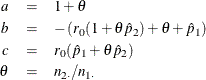
For more information, see Farrington and Manning (1990, p. 1454) and Miettinen and Nurminen (1985, p. 217).
Likelihood Ratio Confidence Limits
Likelihood ratio (profile likelihood) confidence limits for the relative risk are computed by inverting likelihood ratio tests.
The likelihood ratio test statistic for the null hypothesis that the relative risk ratio is can be expressed as
![\[ G^2(r_0) ~ = ~ 2 ~ \bigl ( n_{11} \ln ( \hat{p}_1 / \tilde{p}_1 ) ~ + ~ n_{12} \ln ( (1-\hat{p}_1) / (1-\tilde{p}_1 ) ~ + ~ n_{21} \ln ( \hat{p}_2 / \tilde{p}_2 ) ~ + ~ n_{22} \ln ( (1-\hat{p}_2 / (1-\tilde{p}_2 ) \bigr ) \]](images/procstat_freq0453.png)
where is the observed row i risk ( ) and is the maximum likelihood estimate of the row i risk under the restriction that the relative risk is . Expressions for the maximum likelihood estimates and are given in the subsection "Score Confidence Limits"
in this section. For more information, see Miettinen and Nurminen (1985) and Miettinen (1985, chapter 13).
) and is the maximum likelihood estimate of the row i risk under the restriction that the relative risk is . Expressions for the maximum likelihood estimates and are given in the subsection "Score Confidence Limits"
in this section. For more information, see Miettinen and Nurminen (1985) and Miettinen (1985, chapter 13).
The % likelihood ratio confidence interval for the relative risk consists of all values of for which the test statistic  falls in the acceptance region,
![\[ \{ \theta : G^2(r_0) < \chi ^2_{1, \alpha } \} \]](images/procstat_freq0456.png)
where is the 100th percentile of the chi-square distribution with 1 degree of freedom.
Exact Unconditional Confidence Limits
PROC FREQ computes exact unconditional confidence limits for the relative risk by inverting two separate one-sided tests (tail
method). The size of each test is at most and the confidence coefficient is at least . The exact conditional method, which is described in the section Exact Statistics, does not apply to the relative risk because of a nuisance parameter (Agresti 1992). The unconditional method (which fixes only the row margins of the table) eliminates the nuisance parameter by maximizing the p-value over all possible values of the parameter (Santner and Snell 1980). This computation method is described in the subsection "Exact Unconditional Confidence Limits"
in the section Confidence Limits for the Risk Difference.
By default, PROC FREQ uses the unstandardized relative risk as the test statistic to compute the confidence limits. To ensure that the statistic is defined when there are zero-frequency tables cells, PROC FREQ uses the following modified form of the unstandardized relative risk, which adds 0.5 to the cell and row frequencies (Gart and Nam 1988):
![\[ \hat{r} = \frac{ (n_{11} + 0.5) ~ / ~ (n_{1 \cdot } + 0.5) }{ (n_{21} + 0.5) ~ / ~ (n_{2 \cdot } + 0.5) } \]](images/procstat_freq0457.png)
For more information, see the subsection "Wald Modified Confidence Limits" in this section.
If you specify the RELRISK(METHOD=SCORE) option, PROC FREQ uses the relative risk score statistic as the test statistic to compute the confidence limits (Chan and Zhang 1999). The score statistic is a less discrete statistic than the unstandardized relative risk and produces less conservative confidence limits (Agresti and Min 2001). For more information, see Santner et al. (2007).
The relative risk score statistic (Miettinen and Nurminen 1985; Farrington and Manning 1990) is computed as
![\[ z(r_0) = ( \hat{p}_1 - r_0 \hat{p}_2 ) ~ / ~ \mr{se}(r_0) \]](images/procstat_freq0458.png)
where
![\[ \mr{se}(r_0) = \sqrt { \tilde{p}_1 (1-\tilde{p}_1) / n_{1 \cdot } ~ +~ {r_0}^2 ~ \tilde{p}_2 (1-\tilde{p}_2) / n_{2 \cdot } } \]](images/procstat_freq0459.png)
where and are the maximum likelihood estimates of and under the restriction that the relative risk is . Expressions for the maximum likelihood estimates and are given in the subsection "Score Confidence Limits"
in this section. For more information, see Farrington and Manning (1990, p. 1454) and Miettinen and Nurminen (1985, p. 217).
Relative Risk Tests
PROC FREQ provides tests of equality, noninferiority, superiority, and equivalence for the relative risk. The following analysis methods are available: Wald (which is based on a log transformation), Wald modified, score, and likelihood ratio. You can specify the method by using the METHOD= relrisk-option; by default, PROC FREQ provides Wald tests.
Equality Test
An equality test for the relative risk can be expressed as
![\[ H_0\colon R = r_0 \]](images/procstat_freq0460.png)
versus the alternative
![\[ H_ a\colon R \neq r_0 \]](images/procstat_freq0461.png)
where  denotes the relative risk (for column 1 or column 2) and denotes the null value. You can specify a null value by using the EQUAL(NULL=) relrisk-option; by default, the null value is 1.
The test statistic is computed by the method that you specify; by default, PROC FREQ uses the Wald test. For information about test statistic computation, see the subsections "Wald Test," "Wald Modified Test," "Farrington-Manning (Score) Test," and "Likelihood Ratio Test" in this section.
For the Wald and score methods, the test statistics z have standard normal distributions under the null hypothesis. For the likelihood ratio test, the test statistic  has a chi-square distribution with 1 degree of freedom under the null hypothesis.
When the test statistic z is greater than 0, PROC FREQ displays the right-sided p-value, which is the probability of a larger value occurring under the null hypothesis. The one-sided p-value can be expressed as
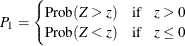
where Z has a standard normal distribution. The two-sided p-value is computed as  .
.
Noninferiority Test
A noninferiority test for the relative risk can be expressed as
![\[ H_0\colon R \leq \delta \]](images/procstat_freq0463.png)
versus the alternative
![\[ H_ a\colon R > \delta \]](images/procstat_freq0464.png)
where denotes the relative risk (for column 1 or column 2) and  denotes the noninferiority margin (limit). You can specify the margin by using the MARGIN= relrisk-option; by default, the noninferiority margin is 0.8. The noninferiority margin for a relative risk test should be less than 1.
Rejection of the null hypothesis indicates that the row 1 risk is not inferior to the row 2 risk. For more information, see
Chow, Shao, and Wang (2008).
denotes the noninferiority margin (limit). You can specify the margin by using the MARGIN= relrisk-option; by default, the noninferiority margin is 0.8. The noninferiority margin for a relative risk test should be less than 1.
Rejection of the null hypothesis indicates that the row 1 risk is not inferior to the row 2 risk. For more information, see
Chow, Shao, and Wang (2008).
The test statistic z is computed by the method that you specify. For information about test statistic computation, see the subsections "Wald Test,"
"Wald Modified Test,"
"Farrington-Manning (Score) Test,"
and "Likelihood Ratio Test"
in this section. The test statistic z is computed by using the noninferiority margin (limit) as the null value of the relative risk. Under the null hypothesis,
the test statistic has a standard normal distribution. The p-value for the noninferiority test is the right-sided p-value (the probability that  ).
).
As part of the noninferiority analysis, PROC FREQ also provides confidence limits for the relative risk. The confidence coefficient
is  % (Schuirmann 1999). The confidence level is determined by the ALPHA=
option in the TABLES statement; by default, ALPHA=0.05, which produces 90% confidence limits for the noninferiority analysis.
You can compare the confidence limits to the value of the noninferiority limit .
% (Schuirmann 1999). The confidence level is determined by the ALPHA=
option in the TABLES statement; by default, ALPHA=0.05, which produces 90% confidence limits for the noninferiority analysis.
You can compare the confidence limits to the value of the noninferiority limit .
Superiority Test
A superiority test for the relative risk can be expressed as
versus the alternative
where denotes the relative risk (for column 1 or column 2) and denotes the superiority margin (limit). You can specify the margin by using the MARGIN= relrisk-option; by default, the superiority margin is 1.25. The superiority margin for a relative risk test should be greater than 1. Rejection
of the null hypothesis indicates that the row 1 risk is superior to the row 2 risk. For more information, see Chow, Shao,
and Wang (2008).
The test statistic z is computed by using the superiority margin (limit) as the null value of the relative risk. Under the null hypothesis, the
test statistic has a standard normal distribution. The p-value for the superiority test is the right-sided p-value (the probability that ).
The computations for the superiority analysis are the same as the computations for the noninferiority analysis, which are described in the subsection "Noninferiority Test" in this section.
Equivalence Test
An equivalence test for the relative risk can be expressed as
![\[ H_0\colon R \leq \delta _{\mi{L}} \hspace{.15in} \mr{or} \hspace{.15in} R \geq \delta _{\mi{U}} \]](images/procstat_freq0466.png)
versus the alternative
![\[ H_ a\colon \delta _{\mi{L}} < R < \delta _{\mi{U}} \]](images/procstat_freq0467.png)
where  is the lower margin and
  is the upper margin. Rejection of the null hypothesis indicates that the two risks are equivalent. For more information,
see Chow, Shao, and Wang (2008).
is the upper margin. Rejection of the null hypothesis indicates that the two risks are equivalent. For more information,
see Chow, Shao, and Wang (2008).
You can specify the margins by using the MARGIN= relrisk-option; by default, the lower margin is 0.8 and the upper margin is 1.25. If you specify a single margin value, PROC FREQ uses this value as the lower margin for the equivalence test and computes the upper margin as the inverse of the lower margin.
PROC FREQ computes two one-sided tests (TOST) for equivalence analysis
(Schuirmann 1987), which include a right-sided test for the lower margin and a left-sided test for the upper margin . The lower test statistic uses the lower margin as the null relative risk value, and the p-value is the right-sided probability ( ). The upper test statistic uses the upper margin as the null value, and the p-value is the left-sided probability (
 ). The overall p-value is taken to be the larger of the two p-values for the lower and upper tests.
The test statistics are computed by the method that you specify. For more information about the test statistic computation, see the subsections "Wald Test," "Wald Modified Test," "Farrington-Manning (Score) Test," and "Likelihood Ratio Test" in this section.
As part of the equivalence analysis, PROC FREQ also provides confidence limits for the relative risk. The confidence coefficient
is % (Schuirmann 1999). The confidence level is determined by the ALPHA=
option in the TABLES statement; by default, ALPHA=0.05, which produces 90% confidence limits for the equivalence analysis.
You can compare the confidence limits to the equivalence limits, which are and .
Wald Test
The Wald test statistic (which is based on a log transformation of the relative risk) is computed as 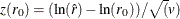 , where is the relative risk estimate (), is the null value of the relative risk, and
![\[ v = \mr{Var}(\ln (\hat{r})) = 1/n_{11} + 1/(n_{21} - 1/n_{1 \cdot } - 1/n_{2 \cdot } \]](images/procstat_freq0471.png)
The null value is determined by the type of test (equality, noninferiority, superiority, or equivalence) and the null or margin values that you specify. The side of the p-value and the interpretation of the test are also determined by the type of test; for more information, see the subsections "Equality Test," "Noninferiority Test," "Superiority Test," and "Equivalence Test" in this section.
Wald Modified Test
The Wald modified test statistic is computed by replacing the with and the with in the relative risk estimator R and the variance v. The test statistic is computed as  , where is the null value of the relative risk,
![\[ \hat{r} = \hat{p}_1 / \hat{p}_2 = \frac{ (n_{11} + 0.5) / (n_{1 \cdot } + 0.5) }{ (n_{21} + 0.5) / (n_{2 \cdot } + 0.5) } \]](images/procstat_freq0473.png)
![\[ v = \mr{Var}(\ln (\hat{r})) = 1/(n_{11} + 0.5) + 1/(n_{21} + 0.5) - 1/(n_{1 \cdot } + 0.5) - 1/(n_{2 \cdot } + 0.5) \]](images/procstat_freq0474.png)
The null value is determined by the type of test (equality, noninferiority, superiority, or equivalence) and the null or margin values that you specify. The side of the p-value and the interpretation of the test are also determined by the type of test; for more information, see the subsections "Equality Test," "Noninferiority Test," "Superiority Test," and "Equivalence Test" in this section.
Farrington-Manning (Score) Test
The relative risk score test statistic (Miettinen and Nurminen 1985; Farrington and Manning 1990) for the null value is computed as
where
where and are the maximum likelihood estimates of and under the null value . Expressions for the maximum likelihood estimates and are given in the subsection "Score Confidence Limits"
in this section.
The null value is determined by the type of test (equality, noninferiority, superiority, or equivalence) and the null or margin values that you specify. The side of the p-value and the interpretation of the test are also determined by the type of test; for more information, see the subsections "Equality Test," "Noninferiority Test," "Superiority Test," and "Equivalence Test" in this section.
Likelihood Ratio Test
The likelihood ratio statistic for the null relative risk value is computed as
where and are the maximum likelihood estimates of and under the null value . Expressions for the maximum likelihood estimates and are given in the subsection "Score Confidence Limits"
in this section. For more information, see Miettinen and Nurminen (1985) and Miettinen (1985, chapter 13).
PROC FREQ computes the likelihood ratio test statistic  for the noninferiority, superiority, and equivalence tests as
  , where the sign is positive if the estimate is greater than the null value (
 ) and negative otherwise (
 ).
).
The null value is determined by the type of test (equality, noninferiority, superiority, or equivalence) and the null or margin values that you specify. The side of the p-value and the interpretation of the test are also determined by the type of test; for more information, see the subsections "Equality Test," "Noninferiority Test," "Superiority Test," and "Equivalence Test" in this section.