The CORR Procedure
- Overview
- Getting Started
-
Syntax

-
DetailsPearson Product-Moment CorrelationSpearman Rank-Order CorrelationKendall’s Tau-b Correlation CoefficientHoeffding Dependence CoefficientPartial CorrelationFisher’s z TransformationPolychoric CorrelationPolyserial CorrelationCronbach’s Coefficient AlphaConfidence and Prediction EllipsesMissing ValuesIn-Database ComputationOutput TablesOutput Data SetsODS Table NamesODS Graphics
-
ExamplesComputing Four Measures of AssociationComputing Correlations between Two Sets of VariablesAnalysis Using Fisher’s z TransformationApplications of Fisher’s z TransformationComputing Polyserial CorrelationsComputing Cronbach’s Coefficient AlphaSaving Correlations in an Output Data SetCreating Scatter PlotsComputing Partial Correlations
- References
The following statements request a correlation analysis and a scatter plot matrix for the variables in the data set Fish1, which was created in Example 2.6.
ods graphics on;
title 'Fish Measurement Data';
proc corr data=fish1 nomiss plots=matrix(histogram);
   var Height Width Length3 Weight3;
run;
ods graphics off;
The “Simple Statistics” table in Output 2.8.1 displays univariate descriptive statistics for analysis variables.
Output 2.8.1: Simple Statistics
| Fish Measurement Data |
| 4 Variables: | Height Width Length3 Weight3 |
|---|
| Simple Statistics | ||||||
|---|---|---|---|---|---|---|
| Variable | N | Mean | Std Dev | Sum | Minimum | Maximum |
| Height | 34 | 15.22057 | 1.98159 | 517.49950 | 11.52000 | 18.95700 |
| Width | 34 | 5.43805 | 0.72967 | 184.89370 | 4.02000 | 6.74970 |
| Length3 | 34 | 38.38529 | 4.21628 | 1305 | 30.00000 | 46.50000 |
| Weight3 | 34 | 8.44751 | 0.97574 | 287.21524 | 6.23168 | 10.00000 |
The “Pearson Correlation Coefficients” table in Output 2.8.2 displays Pearson correlation statistics for pairs of analysis variables.
Output 2.8.2: Pearson Correlation Coefficients
| Pearson Correlation Coefficients, N = 34 Prob > |r| under H0: Rho=0 |
||||||||||||
|---|---|---|---|---|---|---|---|---|---|---|---|---|
| Height | Width | Length3 | Weight3 | |||||||||
| Height |
|
|
|
|
||||||||
| Width |
|
|
|
|
||||||||
| Length3 |
|
|
|
|
||||||||
| Weight3 |
|
|
|
|
||||||||
The variables are highly correlated. For example, the correlation between Height and Width is 0.92632.
The PLOTS=MATRIX(HISTOGRAM) option requests a scatter plot matrix for the VAR statement variables in Output 2.8.3.
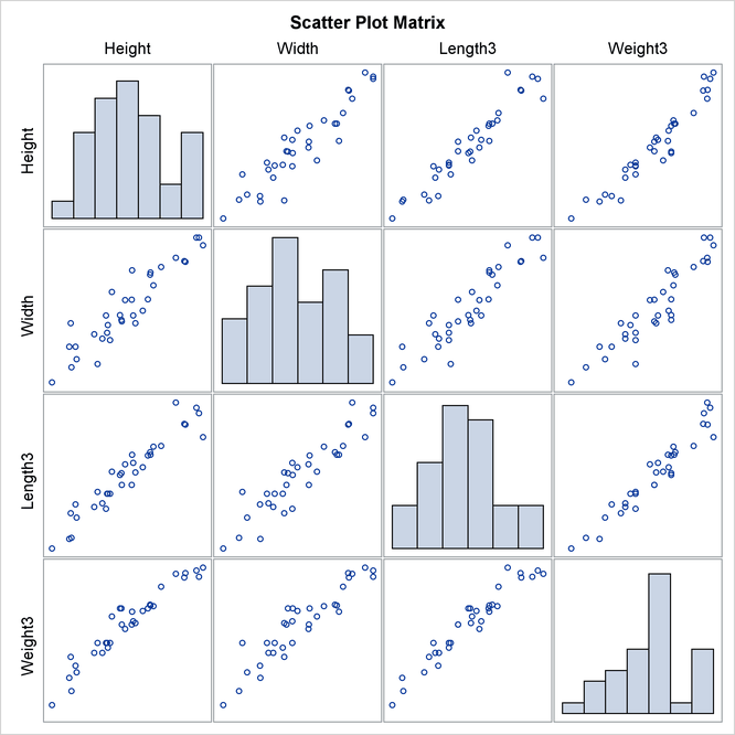
Note that this graphical display is requested by enabling ODS Graphics and by specifying the PLOTS= option. For more information about ODS Graphics, see Chapter 21: Statistical Graphics Using ODS in SAS/STAT 12.3 User's Guide,.
To explore the correlation between Height and Width, the following statements display (in Output 2.8.4) a scatter plot with prediction ellipses for the two variables:
ods graphics on;
proc corr data=fish1 nomiss
          plots=scatter(nvar=2 alpha=.20 .30);
   var Height Width Length3 Weight3;
run;
ods graphics off;
The PLOTS=SCATTER(NVAR=2) option requests a scatter plot for the first two variables in the VAR list. The ALPHA=.20 .30 suboption
requests ![]() and
and ![]() prediction ellipses, respectively.
prediction ellipses, respectively.
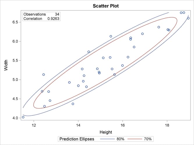
A prediction ellipse is a region for predicting a new observation from the population, assuming bivariate normality. It also
approximates a region that contains a specified percentage of the population. The displayed prediction ellipse is centered
at the means ![]() . For further details, see the section Confidence and Prediction Ellipses.
. For further details, see the section Confidence and Prediction Ellipses.
Note that the following statements also display (in Output 2.8.5) a scatter plot for Height and Width:
ods graphics on;
proc corr data=fish1
          plots=scatter(alpha=.20 .30);
   var Height Width;
run;
ods graphics off;
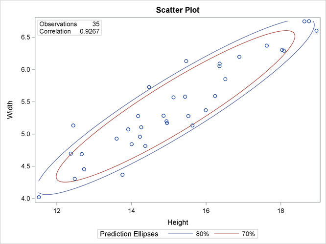
Output 2.8.5 includes the point ![]() , which was excluded from Output 2.8.4 because the observation had a missing value for
, which was excluded from Output 2.8.4 because the observation had a missing value for Weight3. The prediction ellipses in Output 2.8.5 also reflect the inclusion of this observation.
The following statements display (in Output 2.8.6) a scatter plot with confidence ellipses for the mean:
ods graphics on;
title 'Fish Measurement Data';
proc corr data=fish1 nomiss
          plots=scatter(ellipse=confidence nvar=2 alpha=.05 .01);
   var Height Width Length3 Weight3;
run;
ods graphics off;
The NVAR=2 suboption within the PLOTS= option restricts the number of plots created to the first two variables in the VAR
statement, and the ELLIPSE=CONFIDENCE suboption requests confidence ellipses for the mean. The ALPHA=.05 .01 suboption requests
![]() and
and ![]() confidence ellipses, respectively.
confidence ellipses, respectively.
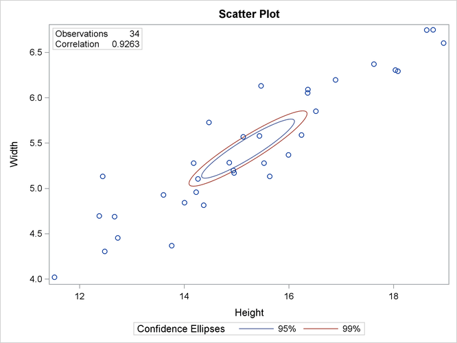
The confidence ellipse for the mean is centered at the means ![]() . For further details, see the section Confidence and Prediction Ellipses.
. For further details, see the section Confidence and Prediction Ellipses.