Example 4.15 Creating a One-Way Comparative Histogram

This example illustrates how to create a comparative histogram. The effective channel length (in microns) is measured for 1225 field effect transistors. The channel lengths (Length) are stored in a data set named Channel, which is partially listed in Output 4.15.1:

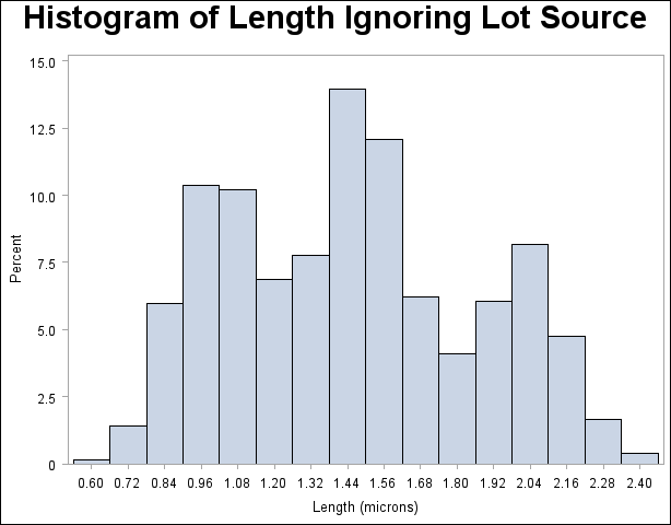
The following statements request a histogram of Length ignoring the lot source:

title 'Histogram of Length Ignoring Lot Source';
proc univariate data=Channel noprint;
   histogram Length;
run;

The resulting histogram is shown in Output 4.15.2.

Output 4.15.2 Histogram for Length Ignoring Lot Source

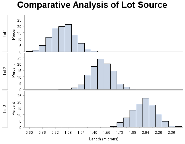
To investigate whether the peaks (modes) in Output 4.15.2 are related to the lot source, you can create a comparative histogram by using Lot as a classification variable. The following statements create the histogram shown in Output 4.15.3:

title 'Comparative Analysis of Lot Source';
proc univariate data=Channel noprint;
   class Lot;
   histogram Length / nrows = 3;
run;

The CLASS statement requests comparisons for each level (distinct value) of the classification variable Lot. The HISTOGRAM statement requests a comparative histogram for the variable Length. The NROWS= option specifies the number of rows per panel in the comparative histogram. By default, comparative histograms are displayed in two rows per panel.

Output 4.15.3 Comparison by Lot Source

Output 4.15.3 reveals that the distributions of Length are similarly distributed except for shifts in mean.

A sample program for this example, uniex09.sas, is available in the SAS Sample Library for Base SAS software.