|
|
Getting Started: CORR Procedure
The following statements create the data set Fitness, which has been altered to contain some missing values:
   *----------------- Data on Physical Fitness -----------------*
   | These measurements were made on men involved in a physical |
   | fitness course at N.C. State University.                   |
   | The variables are Age (years), Weight (kg),                |
   | Runtime (time to run 1.5 miles in minutes), and            |
   | Oxygen (oxygen intake, ml per kg body weight per minute)   |
   | Certain values were changed to missing for the analysis.   |
   *------------------------------------------------------------*;
   data Fitness;
      input Age Weight Oxygen RunTime @@;
      datalines;
   44 89.47 44.609 11.37    40 75.07 45.313 10.07
   44 85.84 54.297  8.65    42 68.15 59.571  8.17
   38 89.02 49.874   .      47 77.45 44.811 11.63
   40 75.98 45.681 11.95    43 81.19 49.091 10.85
   44 81.42 39.442 13.08    38 81.87 60.055  8.63
   44 73.03 50.541 10.13    45 87.66 37.388 14.03
   45 66.45 44.754 11.12    47 79.15 47.273 10.60
   54 83.12 51.855 10.33    49 81.42 49.156  8.95
   51 69.63 40.836 10.95    51 77.91 46.672 10.00
   48 91.63 46.774 10.25    49 73.37   .    10.08
   57 73.37 39.407 12.63    54 79.38 46.080 11.17
   52 76.32 45.441  9.63    50 70.87 54.625  8.92
   51 67.25 45.118 11.08    54 91.63 39.203 12.88
   51 73.71 45.790 10.47    57 59.08 50.545  9.93
   49 76.32   .      .      48 61.24 47.920 11.50
   52 82.78 47.467 10.50
   ;
The following statements invoke the CORR procedure and request a correlation analysis:
ods graphics on;
proc corr data=Fitness plots=matrix(histogram);
run;
ods graphics off;
The "Simple Statistics" table in Figure 2.1 displays univariate statistics for the analysis variables.
Figure 2.1
Univariate Statistics
| Age Weight Oxygen RunTime |
| 31 |
47.67742 |
5.21144 |
1478 |
38.00000 |
57.00000 |
| 31 |
77.44452 |
8.32857 |
2401 |
59.08000 |
91.63000 |
| 29 |
47.22721 |
5.47718 |
1370 |
37.38800 |
60.05500 |
| 29 |
10.67414 |
1.39194 |
309.55000 |
8.17000 |
14.03000 |
By default, all numeric variables not listed in other statements are used in the analysis. Observations with nonmissing values for each variable are used to derive the univariate statistics for that variable.
The "Pearson Correlation Coefficients" table in Figure 2.2 displays the Pearson correlation, the  -value under the null hypothesis of zero correlation, and the number of nonmissing observations for each pair of variables.
Figure 2.2
Pearson Correlation Coefficients
By default, Pearson correlation statistics are computed from observations with nonmissing values for each pair of analysis variables. Figure 2.2 displays a correlation of  0.86843 between Runtime and Oxygen, which is significant with a -value less than 0.0001. That is, there exists an inverse linear relationship between these two variables. As Runtime (time to run 1.5 miles in minutes) increases, Oxygen (oxygen intake, ml per kg body weight per minute) decreases.
This graphical display is requested by specifying the ODS GRAPHICS ON statement and the PLOTS option. For more information about the ODS GRAPHICS statement, see
Chapter 21,
Statistical Graphics Using ODS
(SAS/STAT 9.22 User's Guide).
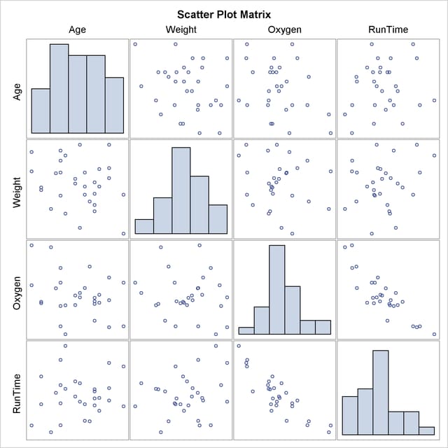
When you use the PLOTS=MATRIX(HISTOGRAM) option, the CORR procedure displays a symmetric matrix plot for the analysis variables in Figure 2.3. The histograms for these analysis variables are also displayed on the diagonal of the matrix plot. This inverse linear relationship between the two variables, Oxygen and Runtime, is also shown in the plot.
Figure 2.3
Symmetric Matrix Plot
Copyright © SAS Institute, Inc. All Rights Reserved.