The HPBIN Procedure

This example shows how you can use the HPBIN procedure to perform pseudo–quantile binning. Consider the following statements:

data bindata;
   do i=1 to 1000;
      x=rannorm(1);
      output;
   end;
run;

proc rank data=bindata out=rankout group=8;
   var x;
   ranks rank_x;
run;

ods graphics on;
proc univariate data=rankout;
   var rank_x;
   histogram;
run;

These statements create a data set that contains 1,000 observations, each generated from a random normal distribution. The histogram for this data set is shown in Figure 3.1.

The pseudo–quantile binning method in the HPBIN procedure can achieve a similar result by using far less computation time. In this case, the time complexity is , where C is a constant and n is the number of observations. When the algorithm runs on the grid, the total amount of computation time is much less. For example, if a cluster has 32 nodes and each node has 24 shared-memory CPUs, then the time complexity is .

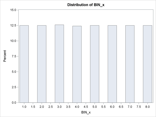
The following statements bin the data by using the PSEUDO_QUANTILE option in the PROC HPBIN statement and generate the histogram for the binning output data. (See Figure 3.2.) This histogram is similar to the one in Figure 3.1.

proc hpbin data=bindata output=binout numbin=8 pseudo_quantile;
   input x;
run;

ods graphics on;
proc univariate data=binout;
   var bin_x;
   histogram;
run;