The HPSUMMARY Procedure

Statistical Computations
Computation of Moment Statistics
PROC HPSUMMARY uses single-pass algorithms to compute the moment statistics (such as mean, variance, skewness, and kurtosis). See the section Keywords and Formulas for the statistical formulas.
The computational details for confidence limits, hypothesis test statistics, and quantile statistics follow.
Confidence Limits
With the statistic-keywords CLM, LCLM, and UCLM, you can compute confidence limits for the mean. A confidence limit is a range (constructed around the
value of a sample statistic) that contains the corresponding true population value with given probability (ALPHA=
) in repeated sampling. A two-sided  % confidence interval for the mean has upper and lower limits
![\[ \bar{x} \pm t_{(1-\alpha /2;\, n-1)} \frac{s}{\sqrt {n}} \]](images/prochp_hpsummary0027.png)
where 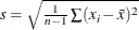 and
and  is the
  critical value of the Student’s t statistic with
  degrees of freedom.
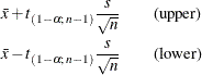
A one-sided % confidence interval is computed as
A two-sided % confidence interval for the standard deviation has lower and upper limits
![\[ s \sqrt {\frac{n - 1}{\chi ^{2}_{(1-\alpha /2;\, n-1)}}}\, , \quad s \sqrt {\frac{n - 1}{\chi ^{2}_{(\alpha /2;\, n-1)}}} \]](images/prochp_hpsummary0032.png)
where  and
and  are the and
  critical values of the chi-square statistic with degrees of freedom. A one-sided % confidence interval is computed by replacing with
  .
.
A % confidence interval for the variance has upper and lower limits that are equal to the squares of the corresponding upper
and lower limits for the standard deviation.
If you use the WEIGHT
statement or the WEIGHT=
option in a VAR
statement and the default value of the VARDEF=
option (which is DF), the % confidence interval for the weighted mean has upper and lower limits
![\[ \bar{y}_ w \pm t_{(1-\alpha /2)} \frac{s_ w}{\sqrt {\displaystyle \sum _{i=1}^{n}w_ i}} \]](images/prochp_hpsummary0037.png)
where  is the weighted mean,
  is the weighted standard deviation,
  is the weight for the ith observation, and
  is the critical value for the Student’s t distribution with degrees of freedom.
Student’s t Test
PROC HPSUMMARY calculates the t statistic as
![\[ t = \frac{\bar{x} - \mu _0}{s / \sqrt {n}} \]](images/prochp_hpsummary0041.png)
where  is the sample mean, n is the number of nonmissing values for a variable, and s is the sample standard deviation. Under the null hypothesis, the population mean equals
  . When the data values are approximately normally distributed, the probability under the null hypothesis of a t statistic as extreme as, or more extreme than, the observed value (the p-value) is obtained from the t distribution with degrees of freedom. For large n, the t statistic is asymptotically equivalent to a z test.
When you use the WEIGHT statement or the WEIGHT= option in a VAR statement and the default value of the VARDEF= option (which is DF), the Student’s t statistic is calculated as
![\[ t_ w = \frac{\bar{y}_ w - \mu _0}{\left.s_ w\middle /\sqrt {\displaystyle \sum _{i=1}^{n}w_ i}\right.} \]](images/prochp_hpsummary0044.png)
where is the weighted mean, is the weighted standard deviation, and is the weight for the ith observation. The  statistic is treated as having a Student’s t distribution with degrees of freedom. If you specify the EXCLNPWGT
option in the PROC HPSUMMARY
statement, then n is the number of nonmissing observations when the value of the WEIGHT variable is positive. By default, n is the number of nonmissing observations for the WEIGHT variable.
statistic is treated as having a Student’s t distribution with degrees of freedom. If you specify the EXCLNPWGT
option in the PROC HPSUMMARY
statement, then n is the number of nonmissing observations when the value of the WEIGHT variable is positive. By default, n is the number of nonmissing observations for the WEIGHT variable.
Quantiles
The options QMETHOD= , QNTLDEF= , and QMARKERS= determine how PROC HPSUMMARY calculates quantiles. The QNTLDEF= option deals with the mathematical definition of a quantile. See the section Quantile and Related Statistics. The QMETHOD= option specifies how PROC HPSUMMARY handles the input data: When QMETHOD=OS, PROC HPSUMMARY reads all data into memory and sorts it by unique value. When QMETHOD=P2, PROC HPSUMMARY accumulates all data into a fixed sample size that is used to approximate the quantile.
If data set A has 100 unique values for a numeric variable X and data set B has 1,000 unique values for numeric variable X, then QMETHOD=OS for data set B requires 10 times as much memory as it does for data set A. If QMETHOD=P2, then both data sets A and B require the same memory space to generate quantiles.
The QMETHOD=P2 technique is based on the piecewise-parabolic ( ) algorithm invented by Jain and Chlamtac (1985). is a one-pass algorithm to determine quantiles for a large data set. It requires a fixed amount of memory for each variable
for each level within the type. However, using simulation studies, reliable estimations of some quantiles (P1, P5, P95, P99)
cannot be possible for some data sets such as data sets with heavily tailed or skewed distributions.
) algorithm invented by Jain and Chlamtac (1985). is a one-pass algorithm to determine quantiles for a large data set. It requires a fixed amount of memory for each variable
for each level within the type. However, using simulation studies, reliable estimations of some quantiles (P1, P5, P95, P99)
cannot be possible for some data sets such as data sets with heavily tailed or skewed distributions.
If the number of observations is less than the QMARKERS= value, then QMETHOD=P2 produces the same results as QMETHOD=OS when QNTLDEF=5. To compute weighted quantiles, you must use QMETHOD=OS.