Statistical Background
Populations and Parameters
Usually, there is a clearly defined set of elements
in which you are interested. This set of elements is called the universe, and a set of values associated with
these elements is called a population of values. The statistical term population has nothing to do with people. A statistical population is a collection
of values, not a collection of people. For example, a universe is
all the students at a particular school, and there could be two populations
of interest: one of height values and one of weight values. Or, a
universe is the set of all widgets manufactured by a particular company,
while the population of values could be the length of time each widget
is used before it fails.
A population of values can be described
in terms of its cumulative distribution function, which gives the proportion of the population less than or equal
to each possible value. A discrete population can also be described
by a probability function,
which gives the proportion of the population equal to each possible
value. A continuous population can often be described by a density function, which is the derivative of
the cumulative distribution function. A density function can be approximated
by a histogram that gives the proportion of the population lying
within each of a series of intervals of values. A probability density
function is like a histogram with an infinite number of infinitely
small intervals.
In
technical literature, when the term distribution is used without qualification, it generally refers to the cumulative
distribution function. In informal writing, distribution sometimes means the density function instead. Often the word distribution is used simply to refer to an abstract
population of values rather than some concrete population. Thus,
the statistical literature refers to many types of abstract distributions,
such as normal distributions, exponential distributions, Cauchy distributions,
and so on. When a phrase such as normal distribution is used, it frequently does not matter whether the cumulative distribution
function or the density function is intended.
It might be
expedient to describe a population in terms of a few measures that
summarize interesting features of the distribution. One such measure,
computed from the population values, is called a parameter. Many different parameters can be defined
to measure different aspects of a distribution.
The most commonly
used parameter is the (arithmetic) mean. If the population contains a finite number of values, then the
population mean is computed as the sum of all the values in the population
divided by the number of elements in the population. For an infinite
population, the concept of the mean is similar but requires more complicated
mathematics.
E(x) denotes the mean of a population of values
symbolized by x, such as height,
where E stands for expected value. You can also consider expected values of derived functions of
the original values. For example, if x represents height, then  is the expected value of height squared, that is,
the mean value of the population obtained by squaring every value
in the population of heights.
is the expected value of height squared, that is,
the mean value of the population obtained by squaring every value
in the population of heights.
is the expected value of height squared, that is,
the mean value of the population obtained by squaring every value
in the population of heights.
Samples and Statistics
It is often impossible to measure all
of the values in a population. A collection of measured values is
called a sample. A mathematical
function of a sample of values is called a statistic. A statistic is to a sample as a parameter is to a population.
It is customary to denote statistics by Roman letters and parameters
by Greek letters. For example, the population mean is often written
as μ, whereas the sample mean is written as  . The field of statistics is largely concerned with the study of the behavior of sample statistics.
. The field of statistics is largely concerned with the study of the behavior of sample statistics.
Samples
can be selected in a variety of ways. Most SAS procedures assume that
the data constitute a simple random sample, which means that the sample was selected in such a way that all
possible samples were equally likely to be selected.
Statistics from
a sample can be used to make inferences, or reasonable guesses, about
the parameters of a population. For example, if you take a random
sample of 30 students from the high school, then the mean height for
those 30 students is a reasonable guess, or estimate, of the mean height of all the students in the high school. Other
statistics, such as the standard error, can provide information about
how good an estimate is likely to be.
For any population parameter,
several statistics can estimate it. Often, however, there is one
particular statistic that is customarily used to estimate a given
parameter. For example, the sample mean is the usual estimator of
the population mean. In the case of the mean, the formulas for the
parameter and the statistic are the same. In other cases, the formula
for a parameter might be different from that of the most commonly
used estimator. The most commonly used estimator is not necessarily
the best estimator in all applications.
Measures of Location
Overview of Measures of Location
Measures of
location include the mean, the median, and the mode. These measures
describe the center of a distribution. In the definitions that follow,
notice that if the entire sample changes by adding a fixed amount
to each observation, then these measures of location are shifted by
the same fixed amount.


The Median
The population median
is the central value, lying above and below half of the population
values. The sample median is the middle value when the data are arranged
in ascending or descending order. For an even number of observations,
the midpoint between the two middle values is usually reported as
the median.
The Mode
The mode is the value
at which the density of the population is at a maximum. Some densities
have more than one local maximum (peak) and are said to be multimodal. The sample mode is the value that
occurs most often in the sample. By default, PROC UNIVARIATE reports
the lowest such value if there is a tie for the most-often-occurring
sample value. PROC UNIVARIATE lists all possible modes when you specify
the MODES option in the PROC statement. If the population is continuous,
then all sample values occur once, and the sample mode has little
use.
Percentiles
Percentiles, including quantiles, quartiles, and the
median, are useful for a detailed study of a distribution. For a set
of measurements arranged in order of magnitude, the pth percentile is the value that has p percent of the measurements below it and (100−p) percent above it. The median is the 50th percentile.
Because it might not be possible to divide your data so that you
get exactly the desired percentile, the UNIVARIATE procedure uses
a more precise definition.
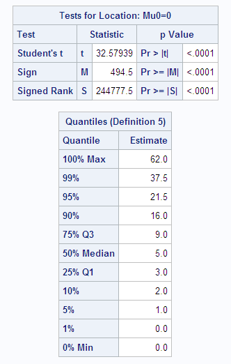
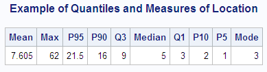
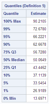
Quantiles
In the following example,
SAS artificially generates the data with a pseudorandom number function.
The UNIVARIATE procedure computes a variety of quantiles and measures
of location, and outputs the values to a SAS data set. A DATA step
then uses the SYMPUT routine to assign the values of the statistics
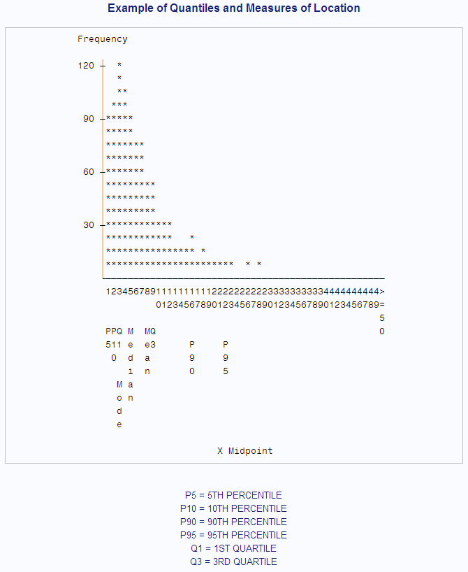
to macro variables. The macro %FORMGEN uses these macro variables
to produce value labels for the FORMAT procedure. PROC CHART uses
the resulting format to display the values of the statistics on a
histogram.
options nodate pageno=1 linesize=80 pagesize=52;

title 'Example of Quantiles and Measures of Location';

data random;
   drop n;
   do n=1 to 1000;
      X=floor(exp(rannor(314159)*.8+1.8));
      output;
   end;
run;

proc univariate data=random nextrobs=0;
   var x;
   output out=location
          mean=Mean mode=Mode median=Median
          q1=Q1 q3=Q3 p5=P5 p10=P10 p90=P90 p95=P95
          max=Max;
run;data _null_;
set location;
call symput('MEAN',round(mean,1));
call symput('MODE',mode);
call symput('MEDIAN',round(median,1));
call symput('Q1',round(q1,1));
call symput('Q3',round(q3,1));
call symput('P5',round(p5,1));
call symput('P10',round(p10,1));
call symput('P90',round(p90,1));
call symput('P95',round(p95,1));
call symput('MAX',min(50,max));
run;
%macro formgen;
%do i=1 %to &max;
%let value=&i;
%if &i=&p5 %then %let value=&value P5;
%if &i=&p10 %then %let value=&value P10;
%if &i=&q1 %then %let value=&value Q1;
%if &i=&mode %then %let value=&value Mode;
%if &i=&median %then %let value=&value Median;
%if &i=&mean %then %let value=&value Mean;
%if &i=&q3 %then %let value=&value Q3;
%if &i=&p90 %then %let value=&value P90;
%if &i=&p95 %then %let value=&value P95;
%if &i=&max %then %let value=>=&value;
&i="&value"
%end;
%mend;
proc format print;
value stat %formgen;
run;
options pagesize=42 linesize=80;
proc chart data=random;
vbar x / midpoints=1 to &max by 1;
format x stat.;
footnote 'P5 = 5TH PERCENTILE';
footnote2 'P10 = 10TH PERCENTILE';
footnote3 'P90 = 90TH PERCENTILE';
footnote4 'P95 = 95TH PERCENTILE';
footnote5 'Q1 = 1ST QUARTILE ';
footnote6 'Q3 = 3RD QUARTILE ';
run;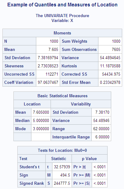
Measures of Variability
Overview of Measures of Variability
Another
group of statistics is important in studying the distribution of a
population. These statistics measure the variability, also called the spread, of values. In the definitions given in
the sections that follow, notice that if the entire sample is changed
by the addition of a fixed amount to each observation, then the values
of these statistics are unchanged. If each observation in the sample
is multiplied by a constant, however, then the values of these statistics
are appropriately rescaled.
The Range
The sample range
is the difference between the largest and smallest values in the sample.
For many populations, at least in statistical theory, the range is
infinite, so the sample range might not tell you much about the population.
The sample range tends to increase as the sample size increases. If
all sample values are multiplied by a constant, then the sample range
is multiplied by the same constant.
The Variance
The population
variance, usually denoted by  , is the expected value of the squared difference
of the values from the population mean:
, is the expected value of the squared difference
of the values from the population mean:
, is the expected value of the squared difference
of the values from the population mean:
The sample variance is denoted by  . The difference between a value and the mean is
called a deviation from the mean. Thus, the variance approximates the mean of the squared deviations.
. The difference between a value and the mean is
called a deviation from the mean. Thus, the variance approximates the mean of the squared deviations.
. The difference between a value and the mean is
called a deviation from the mean. Thus, the variance approximates the mean of the squared deviations.

The Standard Deviation
The
standard deviation is the square root of the variance, or root-mean-square
deviation from the mean, in either a population or a sample. The
usual symbols are σ for the population and s for a sample. The standard deviation is expressed
in the same units as the observations, rather than in squared units.
If all sample values are multiplied by a constant, then the sample
standard deviation is multiplied by the same constant.
Coefficient of Variation
The coefficient of variation is a unitless measure of relative variability.
It is defined as the ratio of the standard deviation to the mean expressed
as a percentage. The coefficient of variation is meaningful only if
the variable is measured on a ratio scale. If all sample values are
multiplied by a constant, then the sample coefficient of variation
remains unchanged.
Measures of Shape
Skewness
The variance is
a measure of the overall size of the deviations from the mean. Since
the formula for the variance squares the deviations, both positive
and negative deviations contribute to the variance in the same way.
In many distributions, positive deviations might tend to be larger
in magnitude than negative deviations, or vice versa. Skewness is a measure of the tendency of the
deviations to be larger in one direction than in the other. For example,
the data in the last example are skewed to the right.

Because the deviations
are cubed rather than squared, the signs of the deviations are maintained.
Cubing the deviations also emphasizes the effects of large deviations.
The formula includes a divisor of  to remove the effect of scale, so multiplying all
values by a constant does not change the skewness. Skewness can thus
be interpreted as a tendency for one tail of the population to be
heavier than the other. Skewness can be positive or negative and is
unbounded.
to remove the effect of scale, so multiplying all
values by a constant does not change the skewness. Skewness can thus
be interpreted as a tendency for one tail of the population to be
heavier than the other. Skewness can be positive or negative and is
unbounded.
to remove the effect of scale, so multiplying all
values by a constant does not change the skewness. Skewness can thus
be interpreted as a tendency for one tail of the population to be
heavier than the other. Skewness can be positive or negative and is
unbounded.
Kurtosis
The heaviness
of the tails of a distribution affects the behavior of many statistics.
Hence it is useful to have a measure of tail heaviness. One such measure
is kurtosis. The population
kurtosis is usually defined as

Because the deviations
are raised to the fourth power, positive and negative deviations make
the same contribution, while large deviations are strongly emphasized.
Because of the divisor  , multiplying each value by a constant has no effect
on kurtosis.
, multiplying each value by a constant has no effect
on kurtosis.
, multiplying each value by a constant has no effect
on kurtosis.
Population kurtosis
must lie between  and
and  , inclusive. If
  represents population skewness and
  represents population kurtosis, then
and , inclusive. If represents population skewness and represents population kurtosis, then
Statistical
literature sometimes reports that kurtosis measures the peakedness of a density. However, heavy tails
have much more influence on kurtosis than does the shape of the distribution
near the mean (Kaplansky 1945; Ali 1974; Johnson, et al. 1980).
Sample skewness and
kurtosis are rather unreliable estimators of the corresponding parameters
in small samples. They are better estimators when your sample is very
large. However, large values of skewness or kurtosis might merit attention
even in small samples because such values indicate that statistical
methods that are based on normality assumptions might be inappropriate.
The Normal Distribution
One
especially important family of theoretical distributions is the normal or Gaussian distribution. A normal distribution is a smooth symmetric function
often referred to as "bell-shaped." Its skewness and kurtosis are
both zero. A normal distribution can be completely specified by only
two parameters: the mean and the standard deviation. Approximately
68% of the values in a normal population are within one standard deviation
of the population mean; approximately 95% of the values are within
two standard deviations of the mean; and about 99.7% are within three
standard deviations. Use of the term normal to describe this particular type of distribution does not imply
that other types of distributions are necessarily abnormal or pathological.
Many statistical methods
are designed under the assumption that the population being sampled
is normally distributed. Nevertheless, most real-life populations
do not have normal distributions. Before using any statistical method
based on normality assumptions, you should consult the statistical
literature to find out how sensitive the method is to nonnormality
and, if necessary, check your sample for evidence of nonnormality.
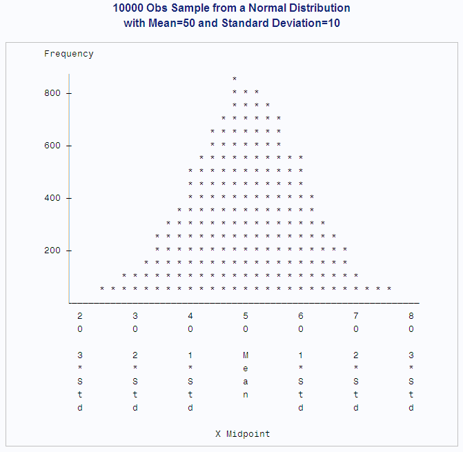
In the following example,
SAS generates a sample from a normal distribution with a mean of 50
and a standard deviation of 10. The UNIVARIATE procedure performs
tests for location and normality. Because the data are from a normal
distribution, all p-values
from the tests for normality are greater than 0.15. The CHART procedure
displays a histogram of the observations. The shape of the histogram
is a bell-like, normal density.
options nodate pageno=1 linesize=80 pagesize=52;

title '10000 Obs Sample from a Normal Distribution';
title2 'with Mean=50 and Standard Deviation=10';

data normaldat;
   drop n;
   do n=1 to 10000;
      X=10*rannor(53124)+50;
      output;
   end;
run;

proc univariate data=normaldat nextrobs=0 normal
                          mu0=50 loccount;
   var x;
run;
proc format;
picture msd
20='20 3*Std' (noedit)
30='30 2*Std' (noedit)
40='40 1*Std' (noedit)
50='50 Mean ' (noedit)
60='60 1*Std' (noedit)
70='70 2*Std' (noedit)
80='80 3*Std' (noedit)
other=' ';
run;
options linesize=80 pagesize=42;
proc chart;
vbar x / midpoints=20 to 80 by 2;
format x msd.;
run;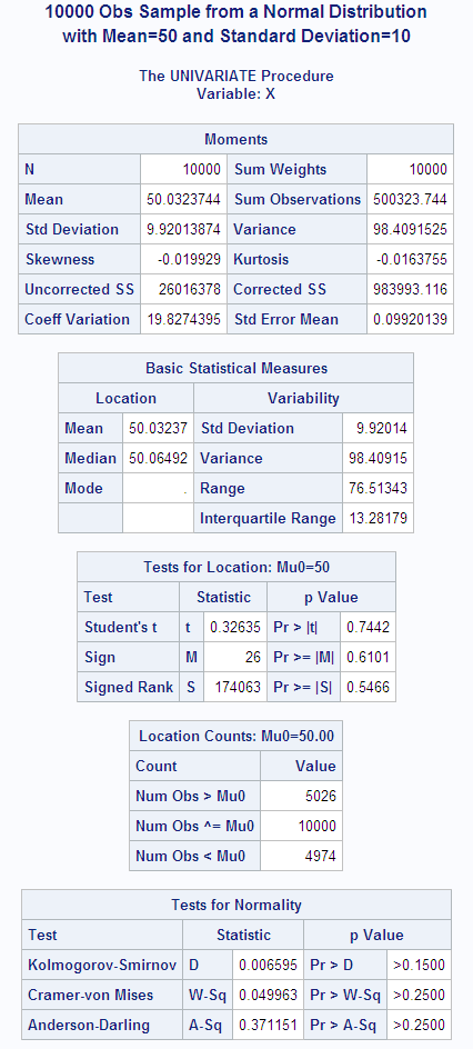
Sampling Distribution of the Mean
If you repeatedly
draw samples of size n from
a population and compute the mean of each sample, then the sample
means themselves have a distribution. Consider a new population consisting
of the means of all the samples that could possibly be drawn from
the original population. The distribution of this new population is
called a sampling distribution.
It can be proven mathematically that if the original population
has mean μ and standard deviation σ, then the sampling
distribution of the mean also has mean μ, but its standard deviation
is  . The standard deviation of the sampling distribution
of the mean is called the standard error of the
mean. The standard error of the mean provides
an indication of the accuracy of a sample mean as an estimator of
the population mean.
. The standard deviation of the sampling distribution
of the mean is called the standard error of the
mean. The standard error of the mean provides
an indication of the accuracy of a sample mean as an estimator of
the population mean.
. The standard deviation of the sampling distribution
of the mean is called the standard error of the
mean. The standard error of the mean provides
an indication of the accuracy of a sample mean as an estimator of
the population mean.
If the original population
has a normal distribution, then the sampling distribution of the mean
is also normal. If the original distribution is not normal but does
not have excessively long tails, then the sampling distribution of
the mean can be approximated by a normal distribution for large sample
sizes.
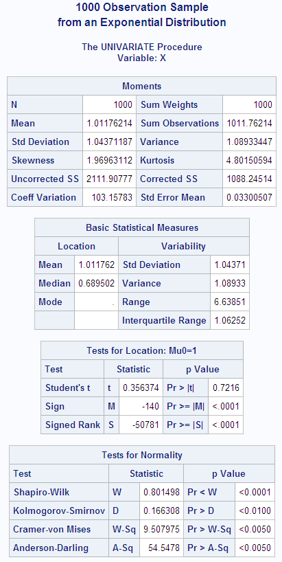
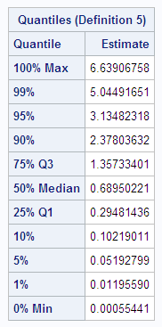
The following example
consists of three separate programs that show how the sampling distribution
of the mean can be approximated by a normal distribution as the sample
size increases. The first DATA step uses the RANEXP function to create
a sample of 1000 observations from an exponential distribution. The
theoretical population mean is 1.00, while the sample mean is 1.01,
to two decimal places. The population standard deviation is 1.00;
the sample standard deviation is 1.04.
The following example
is an example of a nonnormal distribution. The population skewness
is 2.00, which is close to the sample skewness of 1.97. The population
kurtosis is 6.00, but the sample kurtosis is only 4.80.
options nodate pageno=1 linesize=80 pagesize=42;

title '1000 Observation Sample';
title2 'from an Exponential Distribution';

data expodat;
   drop n;
   do n=1 to 1000;
      X=ranexp(18746363);
      output;
   end;
run;
proc format;
    value axisfmt
      .05='0.05'
      .55='0.55'
     1.05='1.05'
     1.55='1.55'
     2.05='2.05'
     2.55='2.55'
     3.05='3.05'
     3.55='3.55'
     4.05='4.05'
     4.55='4.55'
     5.05='5.05'
     5.55='5.55'
     other=' ';
run;

proc chart data=expodat ;
   vbar x / axis=300
            midpoints=0.05 to 5.55 by .1;
   format x axisfmt.;
run;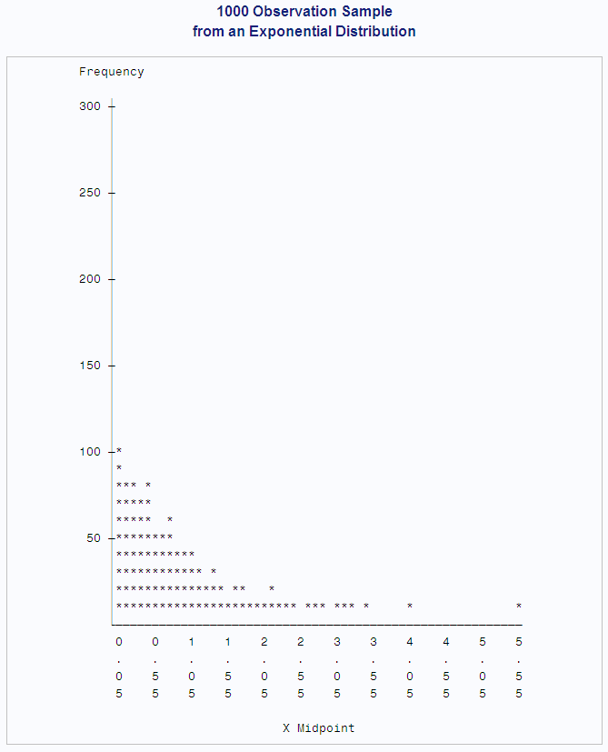
The next DATA step generates
1000 different samples from the same exponential distribution. Each
sample contains ten observations. The MEANS procedure computes the
mean of each sample. In the data set that is created by PROC MEANS,
each observation represents the mean of a sample of ten observations
from an exponential distribution. Thus, the data set is a sample
from the sampling distribution of the mean for an exponential population.
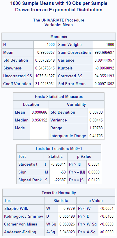
PROC UNIVARIATE displays
statistics for this sample of means. Notice that the mean of the sample
of means is .99, almost the same as the mean of the original population.
Theoretically, the standard deviation of the sampling distribution
is  , whereas the standard deviation of this sample
from the sampling distribution is .30. The skewness (.55) and kurtosis
(-.006) are closer to zero in the sample from the sampling distribution
than in the original sample from the exponential distribution because
the sampling distribution is closer to a normal distribution than
is the original exponential distribution. The CHART procedure displays
a histogram of the 1000-sample means. The shape of the histogram is
much closer to a bell-like, normal density, but it is still distinctly
lopsided.
, whereas the standard deviation of this sample
from the sampling distribution is .30. The skewness (.55) and kurtosis
(-.006) are closer to zero in the sample from the sampling distribution
than in the original sample from the exponential distribution because
the sampling distribution is closer to a normal distribution than
is the original exponential distribution. The CHART procedure displays
a histogram of the 1000-sample means. The shape of the histogram is
much closer to a bell-like, normal density, but it is still distinctly
lopsided.
options nodate pageno=1 linesize=80 pagesize=48;

title '1000 Sample Means with 10 Obs per Sample';
title2 'Drawn from an Exponential Distribution';

data samp10;
   drop n;
   do Sample=1 to 1000;
      do n=1 to 10;
         X=ranexp(433879);
         output;
      end;
   end;

proc means data=samp10 noprint;
   output out=mean10 mean=Mean;
   var x;
   by sample;
run;
proc format;
value axisfmt
.05='0.05'
.55='0.55'
1.05='1.05'
1.55='1.55'
2.05='2.05'
other=' ';
run;
proc chart data=mean10;
vbar mean/axis=300
midpoints=0.05 to 2.05 by .1;
format mean axisfmt.;
run;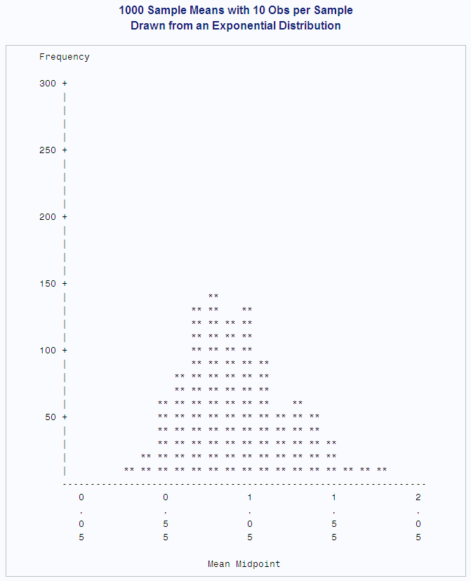
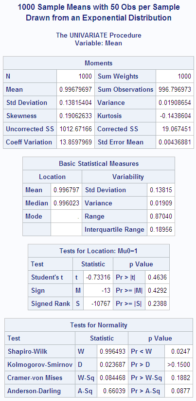
In the following DATA
step, the size of each sample from the exponential distribution is
increased to 50. The standard deviation of the sampling distribution
is smaller than in the previous example because the size of each sample
is larger. Also, the sampling distribution is even closer to a normal
distribution, as can be seen from the histogram and the skewness.
options nodate pageno=1 linesize=80 pagesize=48;

title '1000 Sample Means with 50 Obs per Sample';
title2 'Drawn from an Exponential Distribution';

data samp50;
   drop n;
   do sample=1 to 1000;
      do n=1 to 50;
         X=ranexp(72437213);
         output;
      end;
   end;

proc means data=samp50 noprint;
   output out=mean50 mean=Mean;
   var x;
   by sample;
run;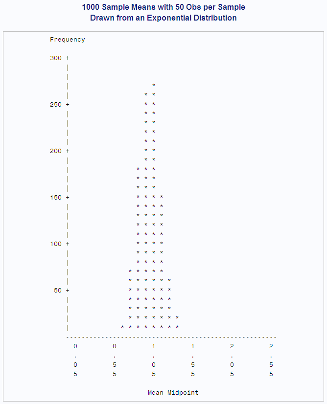
Testing Hypotheses
Defining a Hypothesis
The
purpose of the statistical methods that have been discussed so far
is to estimate a population parameter by means of a sample statistic.
Another class of statistical methods is used for testing hypotheses
about population parameters or for measuring the amount of evidence
against a hypothesis.
Consider the universe
of students in a college. Let the variable X be the number of pounds
by which a student's weight deviates from the ideal weight for a person
of the same sex, height, and build. You want to find out whether
the population of students is, on the average, underweight or overweight.
To this end, you have taken a random sample of X values from nine
students, with results as given in the following DATA step:
You
can define several hypotheses of interest. One hypothesis is that,
on the average, the students are of exactly ideal weight. If μ
represents the population mean of the X values, then you can write
this hypothesis, called the null hypothesis, as  . The other two hypotheses, called alternative hypotheses, are that the students
are underweight on the average,
. The other two hypotheses, called alternative hypotheses, are that the students
are underweight on the average,  , and that the students are overweight on the average,
 .
.
. The other two hypotheses, called alternative hypotheses, are that the students
are underweight on the average, , and that the students are overweight on the average,
.
The null hypothesis
is so called because in many situations it corresponds to the assumption
of “no effect” or “no difference.” However,
this interpretation is not appropriate for all testing problems. The
null hypothesis is like a straw man that can be toppled by statistical
evidence. You decide between the alternative hypotheses according
to which way the straw man falls.
A naive way to approach
this problem would be to look at the sample mean  and decide among the three hypotheses according
to the following rule:
and decide among the three hypotheses according
to the following rule:
and decide among the three hypotheses according
to the following rule:


The trouble with this
approach is that there might be a high probability of making an incorrect
decision. If H0 is true, then you are nearly
certain to make a wrong decision because the chances of  being exactly zero are almost nil. If μ is
slightly less than zero, so that H1 is true,
then there might be nearly a 50% chance that
being exactly zero are almost nil. If μ is
slightly less than zero, so that H1 is true,
then there might be nearly a 50% chance that  will be greater than zero in repeated sampling,
so the chances of incorrectly choosing H2
would also be nearly 50%. Thus, you have a high probability of making
an error if
will be greater than zero in repeated sampling,
so the chances of incorrectly choosing H2
would also be nearly 50%. Thus, you have a high probability of making
an error if  is near zero. In such cases, there is not enough
evidence to make a confident decision, so the best response might
be to reserve judgment until you can obtain more evidence.
is near zero. In such cases, there is not enough
evidence to make a confident decision, so the best response might
be to reserve judgment until you can obtain more evidence.
being exactly zero are almost nil. If μ is
slightly less than zero, so that H1 is true,
then there might be nearly a 50% chance that will be greater than zero in repeated sampling,
so the chances of incorrectly choosing H2
would also be nearly 50%. Thus, you have a high probability of making
an error if is near zero. In such cases, there is not enough
evidence to make a confident decision, so the best response might
be to reserve judgment until you can obtain more evidence.
The question is, how
far from zero must  be for you to be able to make a confident decision?
The answer can be obtained by considering the sampling distribution
of
be for you to be able to make a confident decision?
The answer can be obtained by considering the sampling distribution
of  . If X has an approximately normal distribution,
then
. If X has an approximately normal distribution,
then  has an approximately normal sampling distribution.
The mean of the sampling distribution of
has an approximately normal sampling distribution.
The mean of the sampling distribution of  is μ. Assume temporarily that σ, the
standard deviation of X, is known to be 12. Then the standard error
of
is μ. Assume temporarily that σ, the
standard deviation of X, is known to be 12. Then the standard error
of  for samples of nine observations is
 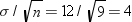 .
.
be for you to be able to make a confident decision?
The answer can be obtained by considering the sampling distribution
of . If X has an approximately normal distribution,
then has an approximately normal sampling distribution.
The mean of the sampling distribution of is μ. Assume temporarily that σ, the
standard deviation of X, is known to be 12. Then the standard error
of for samples of nine observations is .
You know that about
95% of the values from a normal distribution are within two standard
deviations of the mean, so about 95% of the possible samples of nine
X values have a sample mean  between
  and
and  , or between −8 and 8. Consider the chances
of making an error with the following decision rule:
, or between −8 and 8. Consider the chances
of making an error with the following decision rule:
between and , or between −8 and 8. Consider the chances
of making an error with the following decision rule:


If H0 is true, then in about 95% of the possible samples  will be between the critical
values
will be between the critical
values  and 8, so you will reserve judgment. In these cases
the statistical evidence is not strong enough to fell the straw man.
In the other 5% of the samples you will make an error; in 2.5% of
the samples you will incorrectly choose H1,
and in 2.5% you will incorrectly choose H2.
and 8, so you will reserve judgment. In these cases
the statistical evidence is not strong enough to fell the straw man.
In the other 5% of the samples you will make an error; in 2.5% of
the samples you will incorrectly choose H1,
and in 2.5% you will incorrectly choose H2.
will be between the critical
values and 8, so you will reserve judgment. In these cases
the statistical evidence is not strong enough to fell the straw man.
In the other 5% of the samples you will make an error; in 2.5% of
the samples you will incorrectly choose H1,
and in 2.5% you will incorrectly choose H2.
Significance and Power
The probability of rejecting the null hypothesis if it is true is
called the Type I error rate of the statistical test and is typically denoted as  . In this example, an
  value less than
  or greater than 8 is said to be statistically significant at the 5% level. You
can adjust the type I error rate according to your needs by choosing
different critical values. For example, critical values of −4
and 4 would produce a significance level of about 32%, while −12
and 12 would give a type I error rate of about 0.3%.
or greater than 8 is said to be statistically significant at the 5% level. You
can adjust the type I error rate according to your needs by choosing
different critical values. For example, critical values of −4
and 4 would produce a significance level of about 32%, while −12
and 12 would give a type I error rate of about 0.3%.
. In this example, an value less than or greater than 8 is said to be statistically significant at the 5% level. You
can adjust the type I error rate according to your needs by choosing
different critical values. For example, critical values of −4
and 4 would produce a significance level of about 32%, while −12
and 12 would give a type I error rate of about 0.3%.
The decision
rule is a two-tailed test
because the alternative hypotheses allow for population means either
smaller or larger than the value specified in the null hypothesis.
If you were interested only in the possibility of the students being
overweight on the average, then you could use a one-tailed test:


The probability of rejecting the null hypothesis if it is false
is called the power of the
statistical test and is typically denoted as  .
.  is called the Type II error
rate, which is the probability of not rejecting
a false null hypothesis. The power depends on the true value of the
parameter. In the example, assume that the population mean is 4. The
power for detecting H2 is the probability of
getting a sample mean greater than 8. The critical value 8 is one
standard error higher than the population mean 4. The chance of getting
a value at least one standard deviation greater than the mean from
a normal distribution is about 16%, so the power for detecting the
alternative hypothesis H2 is about 16%. If
the population mean were 8, then the power for H2 would be 50%, whereas a population mean of 12 would yield a power
of about 84%.
is called the Type II error
rate, which is the probability of not rejecting
a false null hypothesis. The power depends on the true value of the
parameter. In the example, assume that the population mean is 4. The
power for detecting H2 is the probability of
getting a sample mean greater than 8. The critical value 8 is one
standard error higher than the population mean 4. The chance of getting
a value at least one standard deviation greater than the mean from
a normal distribution is about 16%, so the power for detecting the
alternative hypothesis H2 is about 16%. If
the population mean were 8, then the power for H2 would be 50%, whereas a population mean of 12 would yield a power
of about 84%.
. is called the Type II error
rate, which is the probability of not rejecting
a false null hypothesis. The power depends on the true value of the
parameter. In the example, assume that the population mean is 4. The
power for detecting H2 is the probability of
getting a sample mean greater than 8. The critical value 8 is one
standard error higher than the population mean 4. The chance of getting
a value at least one standard deviation greater than the mean from
a normal distribution is about 16%, so the power for detecting the
alternative hypothesis H2 is about 16%. If
the population mean were 8, then the power for H2 would be 50%, whereas a population mean of 12 would yield a power
of about 84%.
Student's t Distribution
In practice, you usually cannot use any decision rule that uses
a critical value based on σ because you do not usually know
the value of σ. You can, however, use s as an estimate of σ. Consider the following statistic:

This t statistic is the difference between the sample
mean and the hypothesized mean  divided by the estimated standard error of the
mean.
divided by the estimated standard error of the
mean.
divided by the estimated standard error of the
mean.
If the null hypothesis
is true and the population is normally distributed, then the t statistic has what is called a Student's t distribution with  degrees of freedom. This distribution looks very
similar to a normal distribution, but the tails of the Student's t distribution are heavier. As the sample size
gets larger, the sample standard deviation becomes a better estimator
of the population standard deviation, and the t distribution gets closer to a normal distribution.
degrees of freedom. This distribution looks very
similar to a normal distribution, but the tails of the Student's t distribution are heavier. As the sample size
gets larger, the sample standard deviation becomes a better estimator
of the population standard deviation, and the t distribution gets closer to a normal distribution.


The value 2.3 was obtained
from a table of Student's t distribution to give a type I error rate of 5% for 8 (that is,  ) degrees of freedom. Most common statistics texts
contain a table of Student's t distribution. If you do not have a statistics text handy, then you
can use the DATA step and the TINV function to print any values from
the t distribution.
) degrees of freedom. Most common statistics texts
contain a table of Student's t distribution. If you do not have a statistics text handy, then you
can use the DATA step and the TINV function to print any values from
the t distribution.
) degrees of freedom. Most common statistics texts
contain a table of Student's t distribution. If you do not have a statistics text handy, then you
can use the DATA step and the TINV function to print any values from
the t distribution.
By default, PROC UNIVARIATE
computes a t statistic for
the null hypothesis that  , along with related statistics. Use the MU0= option
in the PROC statement to specify another value for the null hypothesis.
, along with related statistics. Use the MU0= option
in the PROC statement to specify another value for the null hypothesis.
, along with related statistics. Use the MU0= option
in the PROC statement to specify another value for the null hypothesis.
This example uses the
data on deviations from normal weight, which consist of nine observations.
First, PROC MEANS computes the t statistic for the null hypothesis that  . Then, the TINV function in a DATA step computes
the value of Student's t distribution
for a two-tailed test at the 5% level of significance and eight degrees
of freedom.
. Then, the TINV function in a DATA step computes
the value of Student's t distribution
for a two-tailed test at the 5% level of significance and eight degrees
of freedom.
. Then, the TINV function in a DATA step computes
the value of Student's t distribution
for a two-tailed test at the 5% level of significance and eight degrees
of freedom.
data devnorm;
   title 'Deviations from Normal Weight';
   input X @@;
   datalines;
-7 -2 1 3 6 10 15 21 30
;

proc means data=devnorm maxdec=3 n mean
           std stderr t probt;
run;

title 'Student''s t Critical Value';

data _null_;
   file print;
   t=tinv(.975,8);
   put t 5.3;
run;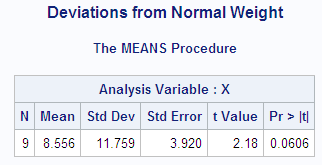

          Deviations from Normal Weight                 1
                      The MEANS Procedure

                     Analysis Variable : X

 N          Mean       Std Dev     Std Error  t Value  Pr > |t|
 --------------------------------------------------------------
 9         8.556        11.759         3.920     2.18    0.0606
 --------------------------------------------------------------
                   Student's t Critical Value                  2
2.306
In the current example,
the value of the t statistic
is 2.18, which is less than the critical t value of 2.3 (for a 5% significance level and eight degrees of freedom).
Thus, at a 5% significance level you must reserve judgment. If you
had elected to use a 10% significance level, then the critical value
of the t distribution would
have been 1.86 and you could have rejected the null hypothesis. The
sample size is so small, however, that the validity of your conclusion
depends strongly on how close the distribution of the population is
to a normal distribution.
Probability Values
Another way to
report the results of a statistical test is to compute a probability value or p-value. A p-value gives the probability
in repeated sampling of obtaining a statistic as far in the directions
specified by the alternative hypothesis as is the value actually observed.
A two-tailed p-value for a t statistic is the probability of obtaining an
absolute t value that is greater
than the observed absolute t value. A one-tailed p-value
for a t statistic for the alternative
hypothesis  is the probability of obtaining a t value greater than the observed t value. Once the p-value is computed, you can perform a hypothesis test by comparing
the p-value with the desired
significance level. If the p-value is less than or equal to the type I error rate of the test,
then the null hypothesis can be rejected. The two-tailed p-value, labeled
is the probability of obtaining a t value greater than the observed t value. Once the p-value is computed, you can perform a hypothesis test by comparing
the p-value with the desired
significance level. If the p-value is less than or equal to the type I error rate of the test,
then the null hypothesis can be rejected. The two-tailed p-value, labeled Pr > |t| in the PROC MEANS output, is .0606, so the null hypothesis could
be rejected at the 10% significance level but not at the 5% level.