Example 4.21 PERT Assumptions and Calculations

This example illustrates the PERT statistical approach. Throughout this chapter, it has been assumed that the activity duration times are precise values determined uniquely. In practice, however, each activity is subject to a number of chance sources of variation and it is impossible to know, a priori, the duration of the activity. The PERT statistical approach is used to include uncertainty about durations in scheduling. For a detailed discussion about various assumptions, techniques, and cautions related to the PERT approach, refer to Moder, Phillips, and Davis (1983) and Elmaghraby (1977). A simple model is used here to illustrate how PROC CPM can incorporate some of these ideas. A more detailed example can be found in SAS/OR Software: Project Management Examples.

Consider the widget manufacturing example. To perform PERT analysis, you need to provide three estimates of activity duration: a pessimistic estimate (tp), an optimistic estimate (to), and a modal estimate (tm). These three estimates are used to obtain a weighted average that is assumed to be a reasonable estimate of the activity duration. The time estimates for the activities must be independent for the analysis to be considered valid. Furthermore, the distribution of activity duration times is purely hypothetical, as no statistical sampling is likely to be feasible on projects of a unique nature to be accomplished at some indeterminate time in the future. Often, the time estimates used are based on past experience with similar projects.

To derive the formula for the mean, you must assume some functional form for the unknown distribution. The well-known Beta distribution is commonly used, as it has the desirable properties of being contained inside a finite interval and can be symmetric or skewed, depending on the location of the mode relative to the optimistic and pessimistic estimates. A linear approximation of the exact formula for the mean of the beta distribution weights the three time estimates as follows:

          (tp + (4*tm) + to) / 6

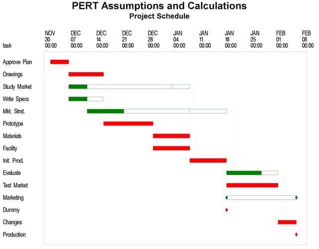
The following program saves the network (AOA format) from Example 4.2 with three estimates of activity durations in a SAS data set. The DATA step also calculates the weighted average duration for each activity. Following the DATA step, PROC CPM is invoked to produce the schedule plotted on a Gantt chart in Output 4.21.1. The E_FINISH time for the final activity in the project contains the mean project completion time based on the duration estimates that are used.

title 'PERT Assumptions and Calculations';
 /* Activity-on-Arc representation of the project
    with three duration estimates */
data widgpert;
   format task $12. ;
   input task & tail head tm tp to;
   dur = (tp + 4*tm + to) / 6;
   datalines;
Approve Plan    1   2    5   7   3
Drawings        2   3   10  11   6
Study Market    2   4    5   7   3
Write Specs     2   3    5   7   3
Prototype       3   5   15  12   9
Mkt. Strat.     4   6   10  11   9
Materials       5   7   10  12   8
Facility        5   7   10  11   9
Init. Prod.     7   8   10  12   8
Evaluate        8   9    9  13   8
Test Market     6   9   14  15  13
Changes         9  10    5   6   4
Production     10  11    0   0   0
Marketing       6  12    0   0   0
Dummy           8   6    0   0   0
;

proc cpm data=widgpert out=sched
     date='1dec03'd;
   tailnode tail;
   headnode head;
   duration dur;
   id task;
   run;

proc sort;
   by e_start;
   run;

goptions vpos=50 hpos=80 border;
proc gantt graphics data=sched;
   chart / compress tailnode=tail headnode=head
           font=swiss height=1.5 nojobnum skip=2
           dur=dur increment=7 nolegend;
           
   id task;
   run;

Some words of caution are worth mentioning with regard to the traditional PERT approach. The estimate of the mean project duration obtained in this instance always underestimates the true value since the length of a critical path is a convex function of the activity durations. The original PERT model developed by Malcolm et al. (1959) provides a way to estimate the variance of the project duration as well as calculating the probabilities of meeting certain target dates and so forth. Their analysis relies on an implicit assumption that you may ignore all activities that are not on the critical path in the deterministic problem that is derived by setting the activity durations equal to the mean value of their distributions. It then applies the Central Limit Theorem to the duration of this critical path and interprets the result as pertaining to the project duration.

Output 4.21.1 PERT Statistical Estimates: Gantt Chart

However, when the activity durations are random variables, each path of the project network is a likely candidate to be the critical path. Every outcome of the activity durations could result in a different longest path. Furthermore, there could be several dependent paths in the network in the sense that they share at least one common arc. Thus, in the most general case, the length of a longest path would be the maximum of a set of, possibly dependent, random variables. Evaluating or approximating the distribution of the longest path, even under very specific distributional assumptions on the activity durations is not a very easy problem. It is not surprising that this topic is the subject of much research.

In view of the inaccuracies that can stem from the original PERT assumptions, many people prefer to resort to the use of Monte Carlo Simulation. Van Slyke (1963) made the first attempt at straightforward simulation to analyze the distribution of the critical path. Refer to Elmaghraby (1977) for a detailed synopsis of the pitfalls of making traditional PERT assumptions and for an introduction to simulation techniques for activity networks.