The Earned Value Management Macros: Charts :: SAS/OR(R) 9.2 User's Guide: Project Management

The Earned Value Management Macros

Charts

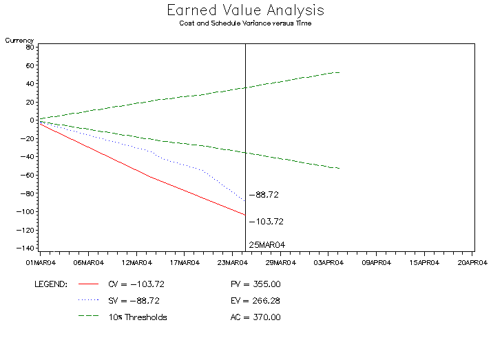
In Figure 9.24, cost and schedule variance are plotted against time using a default invocation of the %EVG_VARIANCE_PLOT macro. Notice that the variances lie outside the plus or minus 10% Planned Value thresholds, which is a cause for concern.

    %evg_variance_plot;

Figure 9.24: CV and SV versus Time Using %EVG_VARIANCE_PLOT

Although not apparent from the preceding chart, as any project nears completion its schedule variance tends toward zero. This is because the earned value eventually converges to the planned value.

Note that the %EVA_METRICS macro must have been called prior to this invocation in order to generate the METRICS= data set.

The cost and schedule variance can also be displayed by activity on a Gantt chart with the %EVG_GANTT_CHART macro, as follows.

    %evg_gantt_chart(
            plansched=software,
            revisesched=software25,
            duration=duration,
            start=start,
            finish=finish,
            activity=activity,
            timenow='25MAR04'd,
            id=wbs cv sv cpi spi,
            height=3,
            scale=20
    );

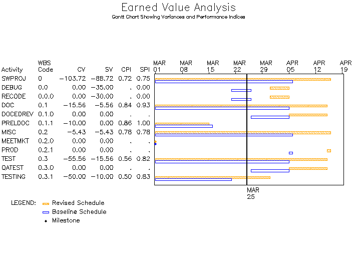
Figure 9.25 depicts cost and schedule variance, in addition to the cost and schedule performance indices, with a Gantt-style schedule. Note that two bars are used to represent each activity. The top bar is the revised schedule and the bottom bar is the baseline schedule.

Figure 9.25: CV and SV by Task Using %EVG_GANTT_CHART

The parameters used in this call to %EVG_GANTT_CHART are described briefly in the following list. More details are given in the section "Syntax".

PLANSCHED= identifies the data set containing the planned schedule.
REVISESCHED= identifies the data set that contains the updated schedule.
ACTIVITY= specifies the activity variable in the PLANSCHED= and REVISESCHED= data sets.
START= specifies the start date or datetime variable in the PLANSCHED= and REVISESCHED= data sets.
FINISH= specifies the finish date or datetime variable in the PLANSCHED= and REVISESCHED= data sets.
DURATION= specifies a duration variable in the PLANSCHED= or REVISESCHED= data set. If the variable is present in both data sets, the REVISESCHED= data set is chosen as the source for the variable values. This variable is only used for differentiating milestones from single day tasks.
TIMENOW= specifies the date or datetime of the updated schedule and costs.
ID= specifies the variable(s) to be included in the Gantt chart.
HEIGHT= specifies a height factor for all text in PROC GANTT. (See the HEIGHT= option for the CHART statement of PROC GANTT ( SAS/OR User's Guide: Project Management, Chapter 4) for more details.)
SCALE= specifies the relative size adjustment of the data columns and chart. (See the SCALE= option for the CHART statement of PROC GANTT ( SAS/OR User's Guide: Project Management, Chapter 4) for more details.)

This macro relies on the output data set (named TASKMETS by default) that is generated by %EVA_TASK_METRICS. The TASKMETRICS= parameter is used by both %EVA_TASK_METRICS and %EVG_GANTT_CHART to specify a different data set name. More details are given in the section "Syntax".

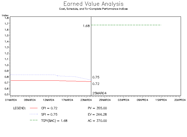
The %EVG_INDEX_PLOT macro is used to generate a line plot of the cost and schedule performance indices, along with the to-complete performance index. The output generated by a default invocation is shown in Figure 9.26. Recall that CPI is the ratio of earned value to actual cost, and SPI is the ratio of earned value to planned value. Also, TCPI $_{\rm bac}$ is the ratio of work remaining to the remaining budget.

    %evg_index_plot;

Figure 9.26: CPI,SPI,and TCPI Using %EVG_INDEX_PLOT

The CPI and SPI plots show a poor cost and schedule performance. Therefore the TCPI $_{\rm bac}$ , an indicator of the performance required to get back on track, is relatively high.

Note that the %EVA_METRICS macro must have been called prior to this invocation in order to generate the METRICS= and SUMMARY= data sets.

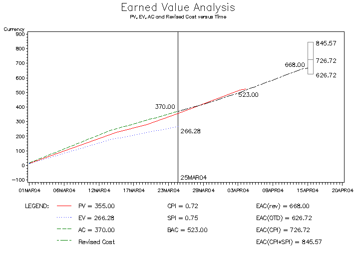
The %EVG_COST_PLOT macro is used to plot the Budgeted Cost of Work Scheduled (or Planned Value), Budgeted Cost of Work Performed (or Earned Value), Actual Cost of Work Performed (or simply Actual Cost), and revised Estimate at Completion (EAC $_{\rm rev}$ ) against time. The output from this macro is shown in Figure 9.27.

    %evg_cost_plot;

Figure 9.27: PV,EV,AC,and EAC $_{\rm rev}$ versus Time Using %EVG_COST_PLOT

The EAC $_{\rm rev}$ value of $668 depicted in Figure 9.27 is the sum of the actual costs so far and the revised cost of the future work. In other words, it is the sum of the "AC Rate" column in the output data set of the %EVA_EARNED_VALUE macro. With the optimistic EAC $_{\rm otd}$ value of $626.72, it is assumed that the remaining work will be completed according to the original budget. A more realistic value of $726.72 is shown for the EAC $_{\rm cpi}$ . Finally, the "upper bound" estimate of $845.57 is given by the EAC $_{\rm cpix spi}$ .

Note that the %EVA_METRICS macro must have been called prior to this invocation in order to generate the METRICS= and SUMMARY= data sets.

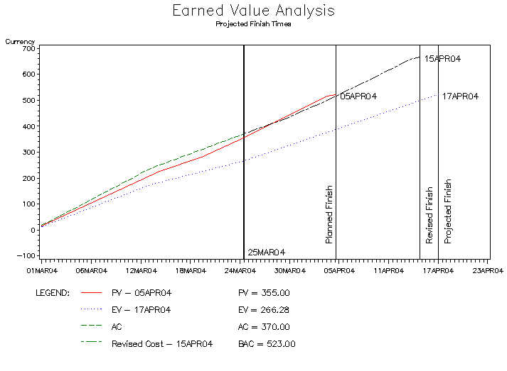
The %EVG_SCHEDULE_PLOT macro can be used to show planned, revised, and projected completion dates as pictured in Figure 9.28.

    %evg_schedule_plot;

Figure 9.28: Projected Completion Dates Using %EVG_SCHEDULE_PLOT

In Figure 9.28, the current date (25MAR04) and planned end date (05APR04) are marked with vertical lines, as is the completion date according to the revised schedule (15APR04). The rightmost vertical line marks the projected finish time based upon the rate at which earned value has accumulated so far. This slope is used to extend the current earned value to the Budget at Completion (BAC) value of $523, providing a prediction of the completion date.

Note that the %EVA_METRICS macro must have been called prior to this invocation in order to generate the METRICS= data set.

Using the software schedule data set as input, the %EVG_WBS_CHART macro can be utilized to produce the Work Breakdown Structure seen in Figure 9.8.

Top of Page