The CPM Procedure

Example 2.31: Resource-Driven Durations and Negative Requirements

A more realistic model for the truck scheduling example can be built if the activities 'First Order' and 'Second Order' are defined to be resource driven. In other words, specify the total amount of work (6 days of work) that is needed from the activity at a pre-specified rate (of 5,000 boxes per day), and allow the choice of machine to dictate the duration of the activity. This modified model is illustrated by the activity data set, TwoOrdersRD, and resource data set, TwoMachinesRD, printed in Output 2.31.1 and Output 2.31.1, respectively. The two orders for greeting cards have a work specification of 6 days if the generic machine Machine (which produces 5,000 boxes a day) is used. The resource data set has a new observation with value 'resrcdur' for the variable obstype. This observation specifies that the resources Machine, Mach1 and Mach2 drive the durations of activities that require them. The third observation in this data set specifies that the second machine is twice as fast as the first one, indicated by the fact that the alternate rate is 0.5. This implies that using the second machine will reduce the activity's duration by 50 percent.

Output 2.31.1: Activity Data Set

Greeting Card Production - Machines 1 and 2 Activity Data Set TwoOrdersRD Obs Activity succ Duration work Machine Mach1 Mach2 numboxes trucks _pattern 1 First Order   1 6 1 . . . . 1 2 Sched truck1 Delivery 1 0 . . . . 10000 . 1 3 Sched truck2 Delivery 2 0 . . . . 10000 . 1 4 Sched truck3 Delivery 3 0 . . . . 10000 . 1 5 Delivery 1   2 . . . . . 1 1 6 Delivery 2   2 . . . . . 1 1 7 Delivery 3   2 . . . . . 1 1 8 Second Order   1 6 1 . . . . 2 9 Sched truck4 Delivery 4 0 . . . . 10000 . 2 10 Sched truck5 Delivery 5 0 . . . . 10000 . 2 11 Sched truck6 Delivery 6 0 . . . . 10000 . 2 12 Delivery 4   2 . . . . . 1 2 13 Delivery 5   2 . . . . . 1 2 14 Delivery 6   2 . . . . . 1 2

Output 2.31.2: Resource Data Set

Greeting Card Production - Machines 1 and 2 Resource Data Set TwoMachinesRD Obs per obstype resid Machine Mach1 Mach2 numboxes trucks 1 . resrcdur   1 1 1.0 . . 2 . restype   1 1 1.0 2 1 3 . altrate Machine . 1 0.5 . . 4 . auxres Mach1 . . . -5000 . 5 . auxres Mach2 . . . -10000 . 6 15AUG04 reslevel   . 1 . . 3 7 24AUG04 reslevel   . 0 1.0 . .

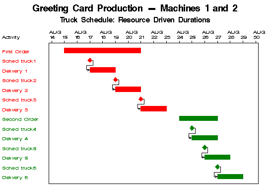
The following statements invoke PROC CPM with the additional specification of the WORK= option. Once again, the CPM procedure allocates one of the two machines for the production, depending on the availability. The Gantt chart is displayed in Figure 2.31.3 and the resource usage data set is printed in Output 2.31.4. As before, the trucks for the first order depart every second day requiring a total of 6 days, while the second order is completed in 3 days. Also, using a resource-driven duration model allows the second activity to be completed in 3 days instead of 6 days, as in the previous example. The resource usage data set indicates that production is stopped as soon as the two orders are filled, avoiding excess inventory.

  
  
    proc cpm data=TwoOrdersRD resin=TwoMachinesRD 
         out=TwoSchedRD rsched=TwoRschedRD resout=TwoRoutRD 
         date='15aug04'd; 
       act      activity; 
       succ     succ; 
       duration duration; 
       resource Machine Mach1 Mach2 numboxes trucks / period=per 
                                             obstype=obstype 
                                             resid=resid work=work 
                                             milestoneresource; 
       id _pattern; 
       run; 
  
    proc sort data=TwoSchedRD; 
       by s_start; 
       run; 
  
    title h=1.5 f=swissb 'Greeting Card Production - Machines 1 and 2'; 
    title2 h=1.2 f=swissb 'Truck Schedule: Resource Driven Durations'; 
    proc gantt data=TwoSchedRD(drop=e_: l:); 
       chart / act=activity succ=succ duration=duration  font=swiss 
               nolegend nojobnum compress pattern=_pattern 
               ctextcols=id scale=4; 
       id activity ; 
       run; 
  
    title2 'Resource Usage Data set: Resource Driven Durations'; 
    proc print data=TwoRoutRD; 
       id _time_; 
       run;
 

Output 2.31.3: Gantt Chart of Schedule

Output 2.31.4: Resource Usage Data Set

Resource Usage Data set: Resource Driven Durations _TIME_ EMachine LMachine RMachine AMachine EMach1 LMach1 RMach1 AMach1 EMach2 LMach2 RMach2 AMach2 Enumboxes Lnumboxes Rnumboxes Anumboxes Etrucks Ltrucks Rtrucks Atrucks 15AUG04 2 2 0 0 0 0 1 0 0 0 0 0 60000 0 -5000 0 6 0 0 3 16AUG04 2 2 0 0 0 0 1 0 0 0 0 0 0 0 -5000 5000 6 0 0 3 17AUG04 2 2 0 0 0 0 1 0 0 0 0 0 0 0 5000 10000 0 0 1 2 18AUG04 2 2 0 0 0 0 1 0 0 0 0 0 0 0 -5000 5000 0 0 1 2 19AUG04 2 2 0 0 0 0 1 0 0 0 0 0 0 60000 5000 10000 0 6 1 2 20AUG04 2 2 0 0 0 0 1 0 0 0 0 0 0 0 -5000 5000 0 6 1 2 21AUG04 0 0 0 0 0 0 0 1 0 0 0 0 0 0 10000 10000 0 0 1 2 22AUG04 0 0 0 0 0 0 0 1 0 0 0 0 0 0 0 0 0 0 1 2 23AUG04 0 0 0 0 0 0 0 1 0 0 0 0 0 0 0 0 0 0 0 3 24AUG04 0 0 0 0 0 0 0 0 0 0 1 0 0 0 -10000 0 0 0 0 3 25AUG04 0 0 0 0 0 0 0 0 0 0 1 0 0 0 0 10000 0 0 1 2 26AUG04 0 0 0 0 0 0 0 0 0 0 1 0 0 0 0 10000 0 0 2 1 27AUG04 0 0 0 0 0 0 0 0 0 0 0 1 0 0 10000 10000 0 0 2 1 28AUG04 0 0 0 0 0 0 0 0 0 0 0 1 0 0 0 0 0 0 1 2 29AUG04 0 0 0 0 0 0 0 0 0 0 0 1 0 0 0 0 0 0 0 3