The OPTMILP Procedure

Example 13.3 Facility Location
This advanced example demonstrates how to warm start PROC OPTMILP by using the PRIMALIN= option. The model is constructed in PROC OPTMODEL and saved in an MPS-format SAS data set for use in PROC OPTMILP. This problem can also be solved from within PROC OPTMODEL; see Chapter 8 for details.
Consider the classical facility location problem. Given a set L of customer locations and a set F of candidate facility sites, you must decide on which sites to build facilities and assign coverage of customer demand to
these sites so as to minimize cost. All customer demand  must be satisfied, and each facility has a demand capacity limit C. The total cost is the sum of the distances
  between facility j and its assigned customer i, plus a fixed charge
  for building a facility at site j. Let
  represent choosing site j to build a facility, and 0 otherwise. Also, let
  represent the assignment of customer i to facility j, and 0 otherwise. This model can be formulated as the following integer linear program:
![\[ \begin{array}{llllll} \min & \displaystyle \sum _{i \in L} \displaystyle \sum _{j \in F} c_{ij} x_{ij} + \displaystyle \sum _{j \in F} f_ j y_ j \\ \mr{s.t.} & \displaystyle \sum _{j \in F} x_{ij} & = & 1 & \forall i \in L & \mr{(assign\_ def)} \\ & x_{ij} & \leq & y_ j & \forall i \in L, j \in F & \mr{(link)}\\ & \displaystyle \sum _{i \in L} d_ i x_{ij} & \leq & Cy_ j & \forall j \in F & \mr{(capacity)} \\ & x_{ij} \in \{ 0,1\} & & & \forall i \in L, j \in F \\ & y_{j} \in \{ 0,1\} & & & \forall j \in F \end{array} \]](images/ormpug_optmilp0075.png)
Constraint (assign_def) ensures that each customer is assigned to exactly one site. Constraint (link) forces a facility to be built if any customer has been assigned to that facility. Finally, constraint (capacity) enforces the capacity limit at each site.
Consider also a variation of this same problem where there is no cost for building a facility. This problem is typically easier to solve than the original problem. For this variant, let the objective be
![\[ \begin{array}{lllll} \min & \displaystyle \sum _{i \in L} \displaystyle \sum _{j \in F} c_{ij} x_{ij} \end{array} \]](images/ormpug_optmilp0076.png)
First, construct a random instance of this problem by using the following DATA steps:
   %let NumCustomers  = 50;
   %let NumSites      = 10;
   %let SiteCapacity  = 35;
   %let MaxDemand     = 10;
   %let xmax          = 200;
   %let ymax          = 100;
   %let seed          = 938;

   /* generate random customer locations */
   data cdata(drop=i);
      length name $8;
      do i = 1 to &NumCustomers;
         name = compress('C'||put(i,best.));
         x = ranuni(&seed) * &xmax;
         y = ranuni(&seed) * &ymax;
         demand = ranuni(&seed) * &MaxDemand;
         output;
      end;
   run;

   /* generate random site locations and fixed charge */
   data sdata(drop=i);
      length name $8;
      do i = 1 to &NumSites;
         name = compress('SITE'||put(i,best.));
         x = ranuni(&seed) * &xmax;
         y = ranuni(&seed) * &ymax;
         fixed_charge = 30 * (abs(&xmax/2-x) + abs(&ymax/2-y));
         output;
      end;
   run;
The following PROC OPTMODEL statements generate the model and define both variants of the cost function:
proc optmodel;
   set <str> CUSTOMERS;
   set <str> SITES init {};
   /* x and y coordinates of CUSTOMERS and SITES */
   num x {CUSTOMERS union SITES};
   num y {CUSTOMERS union SITES};
   num demand {CUSTOMERS};
   num fixed_charge {SITES};
   /* distance from customer i to site j */
   num dist {i in CUSTOMERS, j in SITES}
       = sqrt((x[i] - x[j])^2 + (y[i] - y[j])^2);
   read data cdata into CUSTOMERS=[name] x y demand;
   read data sdata into SITES=[name] x y fixed_charge;
   var Assign {CUSTOMERS, SITES} binary;
   var Build {SITES} binary;
   /* each customer assigned to exactly one site */
   con assign_def {i in CUSTOMERS}:
       sum {j in SITES} Assign[i,j] = 1;
   /* if customer i assigned to site j, then facility must be */
   /* built at j                                              */
   con link {i in CUSTOMERS, j in SITES}:
       Assign[i,j] <= Build[j];
   /* each site can handle at most &SiteCapacity demand */
   con capacity {j in SITES}:
       sum {i in CUSTOMERS} demand[i] * Assign[i,j]
       <= &SiteCapacity * Build[j];
   min CostNoFixedCharge
       = sum {i in CUSTOMERS, j in SITES} dist[i,j] * Assign[i,j];
   save mps nofcdata;
   min CostFixedCharge
       = CostNoFixedCharge
         + sum {j in SITES} fixed_charge[j] * Build[j];
   save mps fcdata;
quit;
First solve the problem for the model with no fixed charge by using the following statements. The first PROC SQL call populates
the macro variables varcostNo. This macro variable displays the objective value when the results are plotted. The second PROC SQL call generates a data
set that is used to plot the results. The information printed in the log by PROC OPTMILP is displayed in Output 13.3.1.
proc optmilp data=nofcdata primalout=nofcout;
run;
proc sql noprint;
   select put(sum(_objcoef_ * _value_),6.1) into :varcostNo
   from nofcout;
quit;
proc sql;
   create table CostNoFixedCharge_Data as
   select
      scan(p._var_,2,'[],') as customer,
      scan(p._var_,3,'[],') as site,
      c.x as xi, c.y as yi, s.x as xj, s.y as yj
   from
      cdata as c,
      sdata as s,
      nofcout(where=(substr(_var_,1,6)='Assign' and
                     round(_value_) = 1)) as p
   where calculated customer = c.name and calculated site = s.name;
quit;
Output 13.3.1: PROC OPTMILP Log for Facility Location with No Fixed Charges
| NOTE: The problem nofcdata has 510 variables (510 binary, 0 integer, 0 free, 0 |
| fixed). |
| NOTE: The problem has 560 constraints (510 LE, 50 EQ, 0 GE, 0 range). |
| NOTE: The problem has 2010 constraint coefficients. |
| NOTE: The MILP presolver value AUTOMATIC is applied. |
| NOTE: The MILP presolver removed 10 variables and 500 constraints. |
| NOTE: The MILP presolver removed 1010 constraint coefficients. |
| NOTE: The MILP presolver modified 0 constraint coefficients. |
| NOTE: The presolved problem has 500 variables, 60 constraints, and 1000 |
| constraint coefficients. |
| NOTE: The MILP solver is called. |
| NOTE: The parallel Branch and Cut algorithm is used. |
| NOTE: The Branch and Cut algorithm is using up to 4 threads. |
| Node Active Sols BestInteger BestBound Gap Time |
| 0 1 2 972.1737321 0 972.2 0 |
| 0 1 2 972.1737321 961.2403449 1.14% 0 |
| 0 1 2 972.1737321 961.2403449 1.14% 0 |
| 0 1 2 972.1737321 961.2403449 1.14% 0 |
| NOTE: The MILP presolver is applied again. |
| 0 1 4 966.4832160 962.9120804 0.37% 0 |
| 0 1 5 966.4832160 966.4832160 0.00% 0 |
| 0 0 5 966.4832160 966.4832160 0.00% 0 |
| NOTE: The MILP solver added 0 cuts with 0 cut coefficients at the root. |
| NOTE: Optimal. |
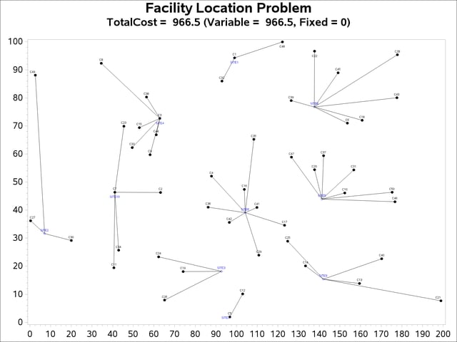
| NOTE: Objective = 966.48321599. |
| NOTE: The data set WORK.NOFCOUT has 510 observations and 8 variables. |
Next, solve the fixed-charge model by using the following statements. Note that the solution to the model with no fixed charge is feasible for the fixed-charge model and should provide a good starting point for PROC OPTMILP. The PRIMALIN= option provides an incumbent solution ("warm start"). The two PROC SQL calls perform the same functions as in the case with no fixed charges. The results from this approach are shown in Output 13.3.2.
proc optmilp data=fcdata primalin=nofcout primalout=fcout;
run;
proc sql noprint;
   select put(sum(_objcoef_ * _value_), 6.1) into :varcost
   from fcout(where=(substr(_var_,1,6)='Assign'));
   select put(sum(_objcoef_ * _value_), 5.1) into :fixcost
   from fcout(where=(substr(_var_,1,5)='Build'));
   select put(sum(_objcoef_ * _value_), 6.1) into :totalcost
   from fcout;
quit;
proc sql;
   create table CostFixedCharge_Data as
   select
      scan(p._var_,2,'[],') as customer,
      scan(p._var_,3,'[],') as site,
      c.x as xi, c.y as yi, s.x as xj, s.y as yj
   from
      cdata as c,
      sdata as s,
      fcout(where=(substr(_var_,1,6)='Assign' and
                   round(_value_) = 1)) as p
   where calculated customer = c.name and calculated site = s.name;
quit;
Output 13.3.2: PROC OPTMILP Log for Facility Location with Fixed Charges, Using Warm Start
| NOTE: The problem fcdata has 510 variables (510 binary, 0 integer, 0 free, 0 |
| fixed). |
| NOTE: The problem has 560 constraints (510 LE, 50 EQ, 0 GE, 0 range). |
| NOTE: The problem has 2010 constraint coefficients. |
| NOTE: The MILP presolver value AUTOMATIC is applied. |
| NOTE: The MILP presolver removed 0 variables and 0 constraints. |
| NOTE: The MILP presolver removed 0 constraint coefficients. |
| NOTE: The MILP presolver modified 0 constraint coefficients. |
| NOTE: The presolved problem has 510 variables, 560 constraints, and 2010 |
| constraint coefficients. |
| NOTE: The MILP solver is called. |
| NOTE: The parallel Branch and Cut algorithm is used. |
| NOTE: The Branch and Cut algorithm is using up to 4 threads. |
| Node Active Sols BestInteger BestBound Gap Time |
| 0 1 3 16070.0150023 0 16070 0 |
| 0 1 3 16070.0150023 9946.2514269 61.57% 0 |
| 0 1 3 16070.0150023 9962.4849932 61.31% 0 |
| 0 1 3 16070.0150023 9971.5893075 61.16% 0 |
| 0 1 3 16070.0150023 9974.5588580 61.11% 0 |
| 0 1 3 16070.0150023 9978.1322942 61.05% 0 |
| 0 1 3 16070.0150023 9978.3312183 61.05% 0 |
| 0 1 3 16070.0150023 9980.4930282 61.01% 0 |
| 0 1 3 16070.0150023 9981.2701907 61.00% 0 |
| 0 1 4 16009.9864088 9981.2701907 60.40% 0 |
| NOTE: The MILP solver added 20 cuts with 631 cut coefficients at the root. |
| 13 8 5 11115.0946280 10027.3840001 10.85% 0 |
| 92 38 6 10986.9615361 10298.3588908 6.69% 0 |
| 101 33 7 10966.7191607 10405.7274389 5.39% 0 |
| 143 14 8 10959.4361909 10789.5675920 1.57% 0 |
| 276 48 9 10950.0345545 10945.3793911 0.04% 0 |
| 348 55 10 10948.4603465 10946.5600201 0.02% 0 |
| 377 40 10 10948.4603465 10947.6598816 0.01% 0 |
| NOTE: Optimal within relative gap. |
| NOTE: Objective = 10948.460346. |
| NOTE: The data set WORK.FCOUT has 510 observations and 8 variables. |
The following two SAS programs produce a plot of the solutions for both variants of the model, using data sets produced by PROC SQL from the PRIMALOUT= data sets produced by PROC OPTMILP.
Note: Execution of this code requires SAS/GRAPH software.
title1 "Facility Location Problem";
title2 "TotalCost = &varcostNo (Variable = &varcostNo, Fixed = 0)";
data csdata;
   set cdata(rename=(y=cy)) sdata(rename=(y=sy));
run;
/* create Annotate data set to draw line between customer and */
/* assigned site                                              */
%annomac;
data anno(drop=xi yi xj yj);
   %SYSTEM(2, 2, 2);
set CostNoFixedCharge_Data(keep=xi yi xj yj);
   %LINE(xi, yi, xj, yj, *, 1, 1);
run;
proc gplot data=csdata anno=anno;
   axis1 label=none order=(0 to &xmax by 10);
   axis2 label=none order=(0 to &ymax by 10);
   symbol1 value=dot interpol=none
      pointlabel=("#name" nodropcollisions height=0.7) cv=black;
   symbol2 value=diamond interpol=none
      pointlabel=("#name" nodropcollisions color=blue height=0.7) cv=blue;
   plot cy*x sy*x / overlay haxis=axis1 vaxis=axis2;
run;
quit;
The output from the first program appears in Output 13.3.3.
Output 13.3.3: Solution Plot for Facility Location with No Fixed Charges
title1 "Facility Location Problem";
title2 "TotalCost = &totalcost (Variable = &varcost, Fixed = &fixcost)";
/* create Annotate data set to draw line between customer and */
/* assigned site                                              */
data anno(drop=xi yi xj yj);
   %SYSTEM(2, 2, 2);
   set CostFixedCharge_Data(keep=xi yi xj yj);
   %LINE(xi, yi, xj, yj, *, 1, 1);
run;
proc gplot data=csdata anno=anno;
   axis1 label=none order=(0 to &xmax by 10);
   axis2 label=none order=(0 to &ymax by 10);
   symbol1 value=dot interpol=none
      pointlabel=("#name" nodropcollisions height=0.7) cv=black;
   symbol2 value=diamond interpol=none
      pointlabel=("#name" nodropcollisions color=blue height=0.7) cv=blue;
   plot cy*x sy*x / overlay haxis=axis1 vaxis=axis2;
run;
quit;
The output from the second program appears in Output 13.3.4.
Output 13.3.4: Solution Plot for Facility Location with Fixed Charges
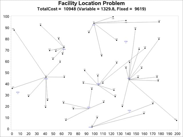
The economic tradeoff for the fixed-charge model forces you to build fewer sites and push more demand to each site.