The Nonlinear Programming Solver

You must specify the COVEST=() option to compute an approximate covariance matrix for the parameter estimates under asymptotic theory for least squares, maximum likelihood, or Bayesian estimation, with or without corrections for degrees of freedom as specified in the VARDEF= option.
The standard form of this class of the problems is one of following:
-
least squares (LSQ):
-
minimum or maximum (MIN/MAX):
For example, two groups of six different forms of covariance matrices (and therefore approximate standard errors) can be computed corresponding to the following two situations, where TERMS is an index set.
-
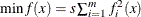
LSQ: The objective function consists solely of a positively scaled sum of squared terms, which means that least squares estimates are being computed:
![\[ \min f(x) = s \sum _{(i,j)\in \mbox{TERMS}} f^2_{ij}(x) \]](images/ormpug_nlpsolver0139.png)
where
 .
.
-
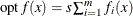
MIN or MAX: The MIN or MAX declaration is specified, and the objective is not in least squares form. Together, these characteristics mean that maximum likelihood or Bayesian estimates are being computed:
![\[ \mr{opt} \, f(x) = s \sum _{(i,j)\in \mbox{TERMS}} f_{ij}(x) \]](images/ormpug_nlpsolver0141.png)
where
 is either
  or
or  and s is arbitrary.
In the preceding section, TERMS is used to denote an arbitrary index set. For example, if your problem is
then TERMS = ![]() , where
, where ![]() is the index set of input data. The following rules apply when you specify your objective function:
is the index set of input data. The following rules apply when you specify your objective function:
-
The terms
 are defined by using the IMPVAR declaration. The i and j values can be partitioned among observation and function indices as needed. Any number of indices can be used, including
non-array indices to implicit variables.
are defined by using the IMPVAR declaration. The i and j values can be partitioned among observation and function indices as needed. Any number of indices can be used, including
non-array indices to implicit variables.
-
The objective consists of a scaled sum of terms (or squared terms for least squares). The scaling, shown as s in the preceding equations, consists of outer multiplication or division by constants of the unscaled sum of terms (or squared terms for least squares). The unary
 or
or  operators can also be used for scaling.
-
Least squares objectives require the scaling to be positive (
). The individual  values are scaled by
  by PROC OPTMODEL.
-
Objectives that are not least squares allow arbitrary scaling. The scale value is distributed to the
values.
-
The summation of terms (or squared terms for least squares) is constructed with the binary
, SUM, and IF-THEN-ELSE operators (where IF-THEN-ELSE must have a first operand that does not depend on variables). The operands
can be terms or a summation of terms (or squared terms for least squares).
-
A squared term is specified as
term^2orterm**2. -
The terms can either be IMPVAR expression or constant expressions (expressions that do not depend on variables). Each IMPVAR element can be referenced at most once in the objective.
-
The number of
terms is determined by counting the nonconstant terms.
The following PROC OPTMODEL statements demonstrate these rules:
var x{VARS};
impvar g{OBS} = ...;
impvar h{OBS} = ...;

/* This objective is okay. */
min z1 = sum{i in OBS} (g[i] + h[i]);

/* This objective is okay. */
min z2 = 0.5*sum{i in OBS} (g[i]^2 + h[i]^2);

/* This objective is okay. It demonstrates multiple levels of scaling. */
min z3 = 3*(sum{i in OBS} (g[i]^2 + h[i]^2))/2;

/* This objective is okay. */
min z4 = (sum{i in OBS} (g[i]^2 + h[i]^2))/2;
Note that the following statements are not accepted:
/* This objective causes an error because individual scaling is not allowed. */
/* (division applies to inner term)                                          */
min z5 = sum{i in OBS} (g[i]^2 + h[i]^2)/2;

/* This objective causes an error because individual scaling is not allowed. */
min z6 = sum{i in OBS} 0.5*g[i]^2;

/* This objective causes an error because the element g[1] is repeated. */
min z7 = g[1] + sum{i in OBS} g[i];
The covariance matrix is always positive semidefinite. For MAX type problems, the covariance matrix is converted to MIN type by using negative Hessian, Jacobian, and function values in the computation. You can use the following options to check for a rank deficiency of the covariance matrix:
-
The ASINGULAR= and MSINGULAR= options enable you to set two singularity criteria for the inversion of the matrix
 that is needed to compute the covariance matrix, when is either the Hessian or one of the crossproduct Jacobian matrices. The singularity criterion that is used for the inversion
is
that is needed to compute the covariance matrix, when is either the Hessian or one of the crossproduct Jacobian matrices. The singularity criterion that is used for the inversion
is
![\[ |d_{j,j}| \le \max (\Argument{asing}, \Argument{msing} \times \max (|A_{1,1}|,\ldots ,|A_{n,n}|)) \]](images/ormpug_nlpsolver0153.png)
where
 is the diagonal pivot of the matrix , and asing and msing are the specified values of the ASINGULAR=
and MSINGULAR=
options, respectively.
is the diagonal pivot of the matrix , and asing and msing are the specified values of the ASINGULAR=
and MSINGULAR=
options, respectively.
-
If the matrix
is found to be singular, the NLP solver computes a generalized inverse that satisfies Moore-Penrose conditions. The generalized inverse is computed using the computationally expensive but numerically stable eigenvalue decomposition,  , where
  is the orthogonal matrix of eigenvectors and
  is the diagonal matrix of eigenvalues,
  . The generalized inverse of is set to
![\[ A^- = Z \Lambda ^- Z^ T \]](images/ormpug_nlpsolver0159.png)
where the diagonal matrix
 is defined as follows, where covsing is the specified value of the COVSING=
option:
is defined as follows, where covsing is the specified value of the COVSING=
option: ![\[ \lambda ^-_ i = \left\{ \begin{array}{ll} 1 / \lambda _ i & \mbox{if $|\lambda _ i| > \Argument{covsing}$} \\ 0 & \mbox{if $|\lambda _ i| \le \Argument{covsing}$} \end{array} \right. \]](images/ormpug_nlpsolver0161.png)
If the COVSING= option is not specified, then the default is
 , where asing and msing are the specified values of the ASINGULAR=
and MSINGULAR=
options, respectively.
, where asing and msing are the specified values of the ASINGULAR=
and MSINGULAR=
options, respectively.
For problems of the MIN or LSQ type, the matrices that are used to compute the covariance matrix are
where ![]() is defined in the standard form of the covariance matrix problem. Note that when some
is defined in the standard form of the covariance matrix problem. Note that when some ![]() are 0,
are 0, ![]() is computed as a generalized inverse.
is computed as a generalized inverse.
For unconstrained minimization, the formulas of the six types of covariance matrices are given in Table 10.2. The value of d in the table depends on the VARDEF= option and the values of the NDF= and NTERMS= options, ndf and nterms, respectively, as follows:
The value of ![]() depends on the specification of the SIGSQ=
option and on the value of d,
depends on the specification of the SIGSQ=
option and on the value of d,
where ![]() is the value of the objective function at the optimal solution
is the value of the objective function at the optimal solution ![]() .
.
Because of the analytic definition, in exact arithmetic the covariance matrix is positive semidefinite at the solution. A warning message is issued if numerical computation does not result in a positive semidefinite matrix. This can happen because round-off error is introduced or the incorrect type of covariance matrix for a specified problem is selected.