The Constraint Programming Solver (Experimental)

Many logic-based puzzles can be formulated as CSPs. Several such puzzles are shown in this example.
Sudoku is a logic-based, combinatorial number-placement puzzle that uses a partially filled 9 × 9 grid. The objective is to fill the grid with the digits 1 to 9 so that each column, each row, and each of the nine 3 × 3 blocks contains only one of each digit. Output 6.1.1 shows an example of a sudoku grid.
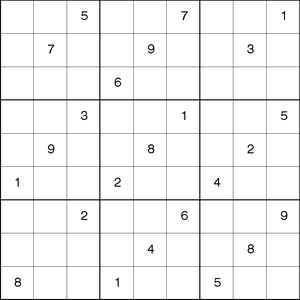
This example illustrates the use of the all-different constraint to solve the preceding sudoku problem. The data set Indata contains the partially filled values for the grid.
data Indata;
   input C1-C9;
   datalines;
. . 5 . . 7 . . 1
. 7 . . 9 . . 3 .
. . . 6 . . . . .
. . 3 . . 1 . . 5
. 9 . . 8 . . 2 .
1 . . 2 . . 4 . .
. . 2 . . 6 . . 9
. . . . 4 . . 8 .
8 . . 1 . . 5 . .
;
Let the variable ![]() represent the value of cell
represent the value of cell ![]() in the grid. The domain of each of these variables is
in the grid. The domain of each of these variables is ![]() . When cell
. When cell ![]() is not missing in the data set,
is not missing in the data set, ![]() is fixed to that value.
is fixed to that value.
Three sets of all-different constraints specify the required rules for each row, each column, and each of the 3 × 3 blocks. The RowCon constraint forces all values in row i to be different, the ColumnCon constraint forces all values in column j to be different, and the BlockCon constraint forces all values in each block to be different.
The following statements express the preceding constraints in PROC OPTMODEL and solve the sudoku puzzle:
proc optmodel;
   /* Declare variables */
   set ROWS = 1..9;
   set COLS = ROWS; /* Use an alias for convenience and clarity */
   var X {ROWS, COLS} >= 1 <= 9 integer;

   /* Nine row constraints */
   con RowCon {i in ROWS}:
      alldiff({j in COLS} X[i,j]);

   /* Nine column constraints */
   con ColCon {j in COLS}:
      alldiff({i in ROWS} X[i,j]);

   /* Nine 3x3 block constraints */
   con BlockCon {s in 0..2, t in 0..2}:
      alldiff({i in 3*s+1..3*s+3, j in 3*t+1..3*t+3} X[i,j]);

   /* Fix variables to cell values */
   /* X[i,j] = c[i,j] if c[i,j] is not missing */
   num c {ROWS, COLS};
   read data indata into [_N_] {j in COLS} <c[_N_,j]=col('C'||j)>;
   for {i in ROWS, j in COLS: c[i,j] ne .}
      fix X[i,j] = c[i,j];

   solve;
quit;
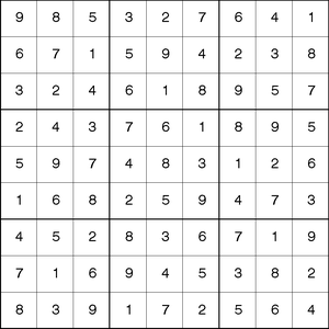
Output 6.1.2 shows the solution.
The basic structure of the classical sudoku problem can easily be extended to formulate more complex puzzles. One such example is the Pi Day sudoku puzzle.
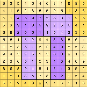
Pi Day is a celebration of the number ![]() that occurs every March 14. In honor of Pi Day, Brainfreeze Puzzles (Riley and Taalman, 2008) celebrates this day with a special 12 × 12 grid sudoku puzzle. The 2008 Pi Day sudoku puzzle is shown in Output 6.1.3.
that occurs every March 14. In honor of Pi Day, Brainfreeze Puzzles (Riley and Taalman, 2008) celebrates this day with a special 12 × 12 grid sudoku puzzle. The 2008 Pi Day sudoku puzzle is shown in Output 6.1.3.
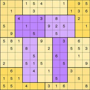
The rules for this puzzle are a little different from the rules for standard sudoku:
-
Rather than using regular 3 × 3 blocks, this puzzle uses jigsaw regions such that highlighted regions in the middle resemble the Greek letter
 . Each jigsaw region consists of 12 contiguous cells.
-
The first 12 digits of
are used instead of the digits 1–9. Each row, column, and jigsaw region contains the first 12 digits of ( ) in some order. In other words, there are no 7s; one each of 2, 4, 6, 8, and 9; two each of 1 and 3; and three 5s.
To generalize the original sudoku model:
-
Replace the expression that calculates the starting and ending cells of a region by an array that maps each cell to one region.
-
Replace the all-different constraints with GCC constraints. GCC constraints describe how often each value can be assigned to a set of variables. Conceptually, an all-different constraint is a specialized GCC constraint in which both the lower bound and the upper bound of every value is 1.
The data set Raw contains the partially filled values for the grid. It contains missing values where the cell does not yet contain a number.
data Raw;
   input C1-C12;
   datalines;
3  .  .  1  5  4  .  .  1  .  9  5
.  1  .  .  3  .  .  .  .  1  3  6
.  .  4  .  .  3  .  8  .  .  2  .
5  .  .  1  .  .  9  2  5  .  .  1
.  9  .  .  5  .  .  5  .  .  .  .
5  8  1  .  .  9  .  .  3  .  6  .
.  5  .  8  .  .  2  .  .  5  5  3
.  .  .  .  5  .  .  6  .  .  1  .
2  .  .  5  1  5  .  .  5  .  .  9
.  6  .  .  4  .  1  .  .  3  .  .
1  5  1  .  .  .  .  5  .  .  5  .
5  5  .  4  .  .  3  1  6  .  .  8
;
The following statements define the GCC constraints in order to find all solutions of the Pi Day sudoku 2008 puzzle:
proc optmodel;
   set ROWS = 1..12;
   /* These declarations are inexpensive and improve clarity: */
   set COLS = ROWS, REGIONS = ROWS, CELLS = ROWS cross COLS;

   /* specify a 12x12 array of region identifiers.
      The spacing is just to make the regions easier to visualize. */
   num region{CELLS} = [
       1  1  1    2  2  2  2  2  2    3  3  3
       1  1  1    2  2  2  2  2  2    3  3  3
       1  1   4  4  4  4    5  5  5  5   3  3
       1  1   4  4  4  4    5  5  5  5   3  3
       1  1   4  4  4  4    5  5  5  5   3  3
       6  6  6   7  7   8  8   9  9  10 10 10
       6  6  6   7  7   8  8   9  9  10 10 10
       6  6  6   7  7   8  8   9  9  10 10 10
       6  6  6   7  7   8  8   9  9  10 10 10
      11 11 11   7  7   8  8   9  9  12 12 12
      11 11 11   7  7   8  8   9  9  12 12 12
      11 11 11 11 11 11     12 12 12 12 12 12 ];

   /* Each area must contain two 1's, two 3's, three 5's, no 7's,
      and one for each of other values from 1 to 9. */
                    /* 1 2 3 4 5 6 7 8 9 */
   num nTimes{1..9} = [2 1 2 1 3 1 0 1 1];
   /* For convenience, create a triplet set version of nTimes.
      In this model, GCC's lower and upper bounds are the same. */
   set N_TIMES = setof{ni in 1..9} <ni,nTimes[ni],nTimes[ni]>;

   /* The number assigned to the ith row and jth column. */
   var X {CELLS} >= 1 <= 9 integer;

   /* X[i,j] = c[i,j] if c[i,j] is not missing */
   num c {CELLS};
   read data raw into [_N_] {j in COLS} <c[_N_,j]=col('C'||j)>;
   for {<i,j> in CELLS: c[i,j] ne .}
      fix X[i,j] = c[i,j];

   con RowCon {i in ROWS}:
      gcc({j in COLS} X[i,j], N_TIMES);

   con ColCon {j in COLS}:
      gcc({i in ROWS} X[i,j], N_TIMES);

   con RegionCon {ri in REGIONS}:
      gcc({<i,j> in CELLS: region[i,j] = ri} X[i,j], N_TIMES);

   solve;
   /* Replicate typical PROC CLP output from PROC OPTMODEL arrays */
   create data pdsout from
      {<i,j> in ROWS cross COLS}<col('X_'||i||'_'||j)=X[i,j]>;
quit;
The only solution of the 2008 Pi Day sudoku puzzle is shown in Output 6.1.4.
Output 6.1.4: Solution to Pi Day Sudoku 2008
| Pi Day Sudoku 2008 |
| Obs | C1 | C2 | C3 | C4 | C5 | C6 | C7 | C8 | C9 | C10 | C11 | C12 |
|---|---|---|---|---|---|---|---|---|---|---|---|---|
| 1 | 3 | 2 | 5 | 1 | 5 | 4 | 6 | 3 | 1 | 8 | 9 | 5 |
| 2 | 4 | 1 | 5 | 2 | 3 | 8 | 5 | 9 | 5 | 1 | 3 | 6 |
| 3 | 6 | 1 | 4 | 5 | 9 | 3 | 5 | 8 | 3 | 1 | 2 | 5 |
| 4 | 5 | 3 | 3 | 1 | 8 | 5 | 9 | 2 | 5 | 6 | 4 | 1 |
| 5 | 8 | 9 | 2 | 6 | 5 | 1 | 1 | 5 | 4 | 3 | 3 | 5 |
| 6 | 5 | 8 | 1 | 5 | 2 | 9 | 4 | 3 | 3 | 5 | 6 | 1 |
| 7 | 1 | 5 | 3 | 8 | 1 | 6 | 2 | 4 | 9 | 5 | 5 | 3 |
| 8 | 9 | 4 | 5 | 3 | 5 | 1 | 5 | 6 | 8 | 2 | 1 | 3 |
| 9 | 2 | 3 | 6 | 5 | 1 | 5 | 3 | 1 | 5 | 4 | 8 | 9 |
| 10 | 3 | 6 | 8 | 9 | 4 | 5 | 1 | 5 | 1 | 3 | 5 | 2 |
| 11 | 1 | 5 | 1 | 3 | 6 | 3 | 8 | 5 | 2 | 9 | 5 | 4 |
| 12 | 5 | 5 | 9 | 4 | 3 | 2 | 3 | 1 | 6 | 5 | 1 | 8 |
The corresponding completed grid is shown in Output 6.1.5.
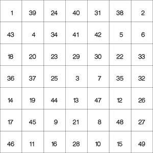
A magic square is an arrangement of the distinct positive integers from 1 to ![]() in an
in an ![]() matrix such that the sum of the numbers of any row, any column, or any main diagonal is the same number, known as the magic
constant. The magic constant of a normal magic square depends only on n and has the value
matrix such that the sum of the numbers of any row, any column, or any main diagonal is the same number, known as the magic
constant. The magic constant of a normal magic square depends only on n and has the value ![]()
This example illustrates the use of the MINRMAXC selection strategy, which is controlled by the VARSELECT= option. In this example, MINRMAXC is the only variable selection strategy that finds a solution to a magic square of size seven within three seconds.
%macro magic(n);
   proc optmodel;
      num n = &n;
      /* magic constant */
      num sum = n*(n^2+1)/2;
      set ROWS = 1..n;
      set COLS = 1..n;

      /* X[i,j] = entry (i,j) */
      var X {ROWS, COLS} >= 1 <= n^2 integer;

      /* row sums */
      con RowCon {i in ROWS}:
         sum {j in COLS} X[i,j] = sum;

      /* column sums */
      con ColCon {j in COLS}:
         sum {i in ROWS} X[i,j] = sum;

      /* diagonal: upper left to lower right */
      con DiagCon:
         sum {i in ROWS} X[i,i] = sum;

      /* diagonal: upper right to lower left */
      con AntidiagCon:
         sum {i in ROWS} X[n+1-i,i] = sum;

      /* symmetry-breaking */
      con BreakRowSymmetry:
         X[1,1] + 1 <= X[n,1];
      con BreakDiagSymmetry:
         X[1,1] + 1 <= X[n,n];
      con BreakAntidiagSymmetry:
         X[1,n] + 1 <= X[n,1];

      con alldiff(X);

      solve with CLP / varselect=minrmaxc maxtime=3;
   quit;
%mend magic;

%magic(7)
The solution is displayed in Output 6.1.6.