The Network Solver (Experimental)
- Overview
- Getting Started
-
Syntax

-
DetailsInput Data for the Network SolverSolving over Subsets of Nodes and Links (Filters)Biconnected Components and Articulation PointsCliqueConnected ComponentsCycleLinear Assignment (Matching)Minimum-Cost Network FlowMinimum CutMinimum Spanning TreeShortest PathTransitive ClosureTraveling Salesman ProblemMacro Variable _OROPTMODEL_
-
ExamplesArticulation Points in a Terrorist NetworkCycle Detection for Kidney Donor ExchangeLinear Assignment Problem for Minimizing Swim TimesLinear Assignment Problem, Sparse Format versus Dense FormatMinimum Spanning Tree for Computer Network TopologyTransitive Closure for Identification of Circular Dependencies in a Bug Tracking SystemTraveling Salesman Tour through US Capital Cities
- References
Consider a cross-country trip where you want to travel the fewest miles to visit all of the capital cities in all US states except Alaska and Hawaii. Finding the optimal route is an instance of the traveling salesman problem, which is described in section Traveling Salesman Problem.
The following PROC SQL statements use the built-in data set maps.uscity to generate a list of the capital cities and their latitude and longitude:
/* Get a list of the state capital cities (with lat and long) */
proc sql;
   create table Cities as
   select unique statecode as state, city, lat, long
      from maps.uscity
      where capital='Y' and statecode not in ('AK' 'PR' 'HI');
quit;
From this list, you can generate a links data set CitiesDist that contains the distances, in miles, between each pair of cities. The distances are calculated by using the SAS function
GEODIST.
/* Create a list of all the possible pairs of cities */
proc sql;
   create table CitiesDist as
   select
      a.city as city1, a.lat as lat1, a.long as long1,
      b.city as city2, b.lat as lat2, b.long as long2,
      geodist(lat1, long1, lat2, long2, 'DM') as distance
      from Cities as a, Cities as b
      where a.city < b.city;
quit;
The following PROC OPTMODEL statements find the optimal tour through each of the capital cities:
/* Find optimal tour by using the network solver */
proc optmodel;
   set<str,str> CAPPAIRS;
   set<str> CAPITALS = union {<i,j> in CAPPAIRS} {i,j};
   num distance{i in CAPITALS, j in CAPITALS: i < j};
   read data CitiesDist into CAPPAIRS=[city1 city2] distance;
   set<str,str> TOUR;
   num order{CAPITALS};

   solve with NETWORK /
      loglevel  = moderate
      links     = (weight=distance)
      tsp
      out       = (order=order tour=TOUR)
   ;

   put (sum{<i,j> in TOUR} distance[i,j]);
   /* Create tour-ordered pairs (rather than input-ordered pairs) */
   str CAPbyOrder{1..card(CAPITALS)};
   for {i in CAPITALS} CAPbyOrder[order[i]] = i;
   set TSPEDGES init
      setof{i in 2..card(CAPITALS)} <CAPbyOrder[i-1],CAPbyOrder[i]>
      union {<CAPbyOrder[card(CAPITALS)],CAPbyOrder[1]>};
   num distance2{<i,j> in TSPEDGES} =
      if i < j then distance[i,j] else distance[j,i];
   create data TSPTourNodes from [node] tsp_order=order;
   create data TSPTourLinks from [city1 city2]=TSPEDGES distance=distance2;
quit;
The progress of the procedure is shown in Output 8.7.1. The total mileage needed to optimally traverse the capital cities is ![]() miles.
miles.
Output 8.7.1: Network Solver Log: Traveling Salesman Tour through US Capital Cities
| NOTE: There were 1176 observations read from the data set WORK.CITIESDIST. |
| NOTE: The experimental Network solver is used. |
| NOTE: The number of nodes in the input graph is 49. |
| NOTE: The number of links in the input graph is 1176. |
| NOTE: Processing the traveling salesman problem. |
| NOTE: The initial TSP heuristics found a tour with cost 10645.918753 using 0.13 |
| (cpu: 0.11) seconds. |
| NOTE: The MILP presolver value NONE is applied. |
| NOTE: The MILP solver is called. |
| Node Active Sols BestInteger BestBound Gap Time |
| 0 1 1 10645.9187534 10040.5139714 6.03% 0 |
| 0 1 2 10645.9187534 10241.6970024 3.95% 0 |
| 0 1 2 10645.9187534 10262.9074205 3.73% 0 |
| 0 1 2 10645.9187534 10293.2995080 3.43% 0 |
| 0 1 2 10645.9187534 10350.0790852 2.86% 0 |
| 0 1 2 10645.9187534 10513.9746901 1.25% 0 |
| 0 1 2 10645.9187534 10529.8732447 1.10% 0 |
| 0 1 2 10645.9187534 10544.6071247 0.96% 0 |
| 0 1 2 10645.9187534 10544.7657451 0.96% 0 |
| 0 1 2 10645.9187534 10590.9748294 0.52% 0 |
| 0 1 2 10645.9187534 10607.8528157 0.36% 0 |
| 0 1 4 10645.9187534 10607.8528157 0.36% 0 |
| NOTE: The MILP solver added 16 cuts with 4753 cut coefficients at the root. |
| 1 1 5 10627.7543183 10607.8528157 0.19% 0 |
| 2 0 5 10627.7543183 10627.7543183 0.00% 0 |
| NOTE: Optimal. |
| NOTE: Objective = 10627.754318. |
| NOTE: Processing the traveling salesman problem used 0.62 (cpu: 0.58) seconds. |
| 10627.754318 |
| NOTE: The data set WORK.TSPTOURNODES has 49 observations and 2 variables. |
| NOTE: The data set WORK.TSPTOURLINKS has 49 observations and 3 variables. |
The following PROC GPROJECT and PROC GMAP statements produce a graphical display of the solution:
/* Merge latitude and longitude */
proc sql;
   /* merge in the lat & long for city1 */
   create table TSPTourLinksAnno1 as
   select unique TSPTourLinks.*, cities.lat as lat1, cities.long as long1
      from TSPTourLinks left join cities
      on TSPTourLinks.city1=cities.city;
   /* merge in the lat & long for city2 */
   create table TSPTourLinksAnno2 as
   select unique TSPTourLinksAnno1.*, cities.lat as lat2, cities.long as long2
      from TSPTourLinksAnno1 left join cities
      on TSPTourLinksAnno1.city2=cities.city;
quit;
/* Create the annotated data set to draw the path on the map
    (convert lat & long degrees to radians, since the map is in radians) */
data anno_path;
   set TSPTourLinksAnno2;
   length function color $8;
   xsys='2'; ysys='2'; hsys='3'; when='a'; anno_flag=1;
   function='move';
   x=atan(1)/45 * long1;
   y=atan(1)/45 * lat1;
   output;
   function='draw';
   color="blue"; size=0.8;
   x=atan(1)/45 * long2;
   y=atan(1)/45 * lat2;
   output;
run;

/* Get a map with only the contiguous 48 states */
data states;
   set maps.states (where=(fipstate(state) not in ('HI' 'AK' 'PR')));
run;

data combined;
   set states anno_path;
run;
/* Project the map and annotate the data */
proc gproject data=combined out=combined dupok;
   id state;
run;

data states anno_path;
   set combined;
   if anno_flag=1 then output anno_path;
   else                output states;
run;
/* Get a list of the endpoints locations */
proc sql;
   create table anno_dots as
   select unique x, y from anno_path;
quit;
/* Create the final annotate data set */
data anno_dots;
   set anno_dots;
   length function color $8;
   xsys='2'; ysys='2'; when='a'; hsys='3';
   function='pie';
   rotate=360; size=0.8; style='psolid'; color="red";
   output;
   style='pempty'; color="black";
   output;
run;
/* Generate the map with GMAP */
pattern1 v=s c=cxccffcc repeat=100;
proc gmap data=states map=states anno=anno_path all;
   id state;
   choro state / levels=1 nolegend coutline=black
                 anno=anno_dots des='' name="tsp";
run;
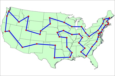
The minimal cost tour through the capital cities is shown on the US map in Output 8.7.2.
The data set TSPTourLinks contains the links in the optimal tour. To display the links in the order they are to be visited, you can use the following
DATA step:
/* Create the directed optimal tour */
data TSPTourLinksDirected(drop=next);
   set TSPTourLinks;
   retain next;
   if _N_ ne 1 and city1 ne next then do;
      city2 = city1;
      city1 = next;
   end;
   next = city2;
run;
The data set TSPTourLinksDirected is shown in Output 8.7.3.
Output 8.7.3: Links in the Optimal Traveling Salesman Tour
| city1 | city2 | distance |
|---|---|---|
| Montgomery | Tallahassee | 177.14 |
| Tallahassee | Columbia | 311.23 |
| Columbia | Raleigh | 182.99 |
| Raleigh | Richmond | 135.58 |
| Richmond | Washington | 97.96 |
| Washington | Annapolis | 27.89 |
| Annapolis | Dover | 54.01 |
| Dover | Trenton | 83.88 |
| Trenton | Hartford | 151.65 |
| Hartford | Providence | 65.56 |
| Providence | Boston | 38.41 |
| Boston | Concord | 66.30 |
| Concord | Augusta | 117.36 |
| Augusta | Montpelier | 139.32 |
| Montpelier | Albany | 126.19 |
| Albany | Harrisburg | 230.24 |
| Harrisburg | Charleston | 287.34 |
| Charleston | Columbus | 134.64 |
| Columbus | Lansing | 205.08 |
| Lansing | Madison | 246.88 |
| Madison | Saint Paul | 226.25 |
| Saint Paul | Bismarck | 391.25 |
| Bismarck | Pierre | 170.27 |
| Pierre | Cheyenne | 317.90 |
| Cheyenne | Denver | 98.33 |
| Denver | Salt Lake City | 373.05 |
| Salt Lake City | Helena | 403.40 |
| Helena | Boise City | 291.20 |
| Boise City | Olympia | 401.31 |
| Olympia | Salem | 146.00 |
| Salem | Sacramento | 447.40 |
| Sacramento | Carson City | 101.51 |
| Carson City | Phoenix | 577.84 |
| Phoenix | Santa Fe | 378.27 |
| Santa Fe | Oklahoma City | 474.92 |
| Oklahoma City | Austin | 357.38 |
| Austin | Baton Rouge | 394.78 |
| Baton Rouge | Jackson | 139.75 |
| Jackson | Little Rock | 206.87 |
| Little Rock | Jefferson City | 264.75 |
| Jefferson City | Topeka | 191.67 |
| Topeka | Lincoln | 132.94 |
| Lincoln | Des Moines | 168.10 |
| Des Moines | Springfield | 243.02 |
| Springfield | Indianapolis | 186.46 |
| Indianapolis | Frankfort | 129.90 |
| Frankfort | Nashville-Davidson | 175.58 |
| Nashville-Davidson | Atlanta | 212.61 |
| Atlanta | Montgomery | 145.39 |
| 10,627.75 |