The Mixed Integer Linear Programming Solver

Example 7.3 Facility Location
Consider the classic facility location problem. Given a set L of customer locations and a set F of candidate facility sites, you must decide on which sites to build facilities and assign coverage of customer demand to
these sites so as to minimize cost. All customer demand ![]() must be satisfied, and each facility has a demand capacity limit C. The total cost is the sum of the distances
must be satisfied, and each facility has a demand capacity limit C. The total cost is the sum of the distances ![]() between facility j and its assigned customer i, plus a fixed charge
between facility j and its assigned customer i, plus a fixed charge ![]() for building a facility at site j. Let
for building a facility at site j. Let ![]() represent choosing site j to build a facility, and 0 otherwise. Also, let
represent choosing site j to build a facility, and 0 otherwise. Also, let ![]() represent the assignment of customer i to facility j, and 0 otherwise. This model can be formulated as the following integer linear program:
represent the assignment of customer i to facility j, and 0 otherwise. This model can be formulated as the following integer linear program:
![\[ \begin{array}{llllll} \min & \displaystyle \sum _{i \in L} \displaystyle \sum _{j \in F} c_{ij} x_{ij} + \displaystyle \sum _{j \in F} f_ j y_ j \\ \mr {s.t.} & \displaystyle \sum _{j \in F} x_{ij} & = & 1 & \forall i \in L & \mr {(assign\_ def)} \\ & x_{ij} & \leq & y_ j & \forall i \in L, j \in F & \mr {(link)}\\ & \displaystyle \sum _{i \in L} d_ i x_{ij} & \leq & Cy_ j & \forall j \in F & \mr {(capacity)} \\ & x_{ij} \in \{ 0,1\} & & & \forall i \in L, j \in F \\ & y_{j} \in \{ 0,1\} & & & \forall j \in F \end{array} \]](images/ormpug_milpsolver0080.png) |
Constraint (assign_def) ensures that each customer is assigned to exactly one site. Constraint (link) forces a facility to be built if any customer has been assigned to that facility. Finally, constraint (capacity) enforces the capacity limit at each site.
Consider also a variation of this same problem where there is no cost for building a facility. This problem is typically easier to solve than the original problem. For this variant, let the objective be
|
|
First, construct a random instance of this problem by using the following DATA steps:
title 'Facility Location Problem';
%let NumCustomers  = 50;
%let NumSites      = 10;
%let SiteCapacity  = 35;
%let MaxDemand     = 10;
%let xmax          = 200;
%let ymax          = 100;
%let seed          = 938;

/* generate random customer locations */
data cdata(drop=i);
   length name $8;
   do i = 1 to &NumCustomers;
      name = compress('C'||put(i,best.));
      x = ranuni(&seed) * &xmax;
      y = ranuni(&seed) * &ymax;
      demand = ranuni(&seed) * &MaxDemand;
      output;
   end;
run;

/* generate random site locations and fixed charge */
data sdata(drop=i);
   length name $8;
   do i = 1 to &NumSites;
      name = compress('SITE'||put(i,best.));
      x = ranuni(&seed) * &xmax;
      y = ranuni(&seed) * &ymax;
      fixed_charge = 30 * (abs(&xmax/2-x) + abs(&ymax/2-y));
      output;
   end;
run;
The following PROC OPTMODEL statements first generate and solve the model with the no-fixed-charge variant of the cost function. Next, they solve the fixed-charge model. Note that the solution to the model with no fixed charge is feasible for the fixed-charge model and should provide a good starting point for the MILP solver. Use the PRIMALIN option to provide an incumbent solution (warm start).
proc optmodel;
   set <str> CUSTOMERS;
   set <str> SITES init {};
   /* x and y coordinates of CUSTOMERS and SITES */
   num x {CUSTOMERS union SITES};
   num y {CUSTOMERS union SITES};
   num demand {CUSTOMERS};
   num fixed_charge {SITES};

   /* distance from customer i to site j */
   num dist {i in CUSTOMERS, j in SITES}
       = sqrt((x[i] - x[j])^2 + (y[i] - y[j])^2);

   read data cdata into CUSTOMERS=[name] x y demand;
   read data sdata into SITES=[name] x y fixed_charge;

   var Assign {CUSTOMERS, SITES} binary;
   var Build {SITES} binary;

   min CostNoFixedCharge
       = sum {i in CUSTOMERS, j in SITES} dist[i,j] * Assign[i,j];
   min CostFixedCharge
       = CostNoFixedCharge + sum {j in SITES} fixed_charge[j] * Build[j];

   /* each customer assigned to exactly one site */
   con assign_def {i in CUSTOMERS}:
      sum {j in SITES} Assign[i,j] = 1;

   /* if customer i assigned to site j, then facility must be built at j */
   con link {i in CUSTOMERS, j in SITES}:
      Assign[i,j] <= Build[j];

   /* each site can handle at most &SiteCapacity demand */
   con capacity {j in SITES}:
      sum {i in CUSTOMERS} demand[i] * Assign[i,j] <=
         &SiteCapacity * Build[j];

   /* solve the MILP with no fixed charges */
   solve obj CostNoFixedCharge with milp / logfreq = 500;

   /* clean up the solution */
   for {i in CUSTOMERS, j in SITES} Assign[i,j] = round(Assign[i,j]);
   for {j in SITES} Build[j] = round(Build[j]);

   call symput('varcostNo',put(CostNoFixedCharge,6.1));

   /* create a data set for use by GPLOT */
   create data CostNoFixedCharge_Data from
      [customer site]={i in CUSTOMERS, j in SITES: Assign[i,j] = 1}
      xi=x[i] yi=y[i] xj=x[j] yj=y[j];

   /* solve the MILP, with fixed charges with warm start */
   solve obj CostFixedCharge with milp / primalin logfreq = 500;

   /* clean up the solution */
   for {i in CUSTOMERS, j in SITES} Assign[i,j] = round(Assign[i,j]);
   for {j in SITES} Build[j] = round(Build[j]);

   num varcost = sum {i in CUSTOMERS, j in SITES} dist[i,j] * Assign[i,j].sol;
   num fixcost = sum {j in SITES} fixed_charge[j] * Build[j].sol;
   call symput('varcost', put(varcost,6.1));
   call symput('fixcost', put(fixcost,5.1));
   call symput('totalcost', put(CostFixedCharge,6.1));

   /* create a data set for use by GPLOT */
   create data CostFixedCharge_Data from
      [customer site]={i in CUSTOMERS, j in SITES: Assign[i,j] = 1}
      xi=x[i] yi=y[i] xj=x[j] yj=y[j];
quit;
The information printed in the log for the no-fixed-charge model is displayed in Output 7.3.1.
Output 7.3.1: OPTMODEL Log for Facility Location with No Fixed Charges
| Facility Location Problem |
| NOTE: Problem generation will use 2 threads. |
| NOTE: The problem has 510 variables (0 free, 0 fixed). |
| NOTE: The problem has 510 binary and 0 integer variables. |
| NOTE: The problem has 560 linear constraints (510 LE, 50 EQ, 0 GE, 0 range). |
| NOTE: The problem has 2010 linear constraint coefficients. |
| NOTE: The problem has 0 nonlinear constraints (0 LE, 0 EQ, 0 GE, 0 range). |
| NOTE: The MILP presolver value AUTOMATIC is applied. |
| NOTE: The MILP presolver removed 10 variables and 500 constraints. |
| NOTE: The MILP presolver removed 1010 constraint coefficients. |
| NOTE: The MILP presolver modified 0 constraint coefficients. |
| NOTE: The presolved problem has 500 variables, 60 constraints, and 1000 |
| constraint coefficients. |
| NOTE: The MILP solver is called. |
| Node Active Sols BestInteger BestBound Gap Time |
| 0 1 2 972.1737321 0 972.2 0 |
| 0 1 2 972.1737321 961.2403449 1.14% 0 |
| 0 1 3 966.4832160 966.4832160 0.00% 0 |
| 0 0 3 966.4832160 966.4832160 0.00% 0 |
| NOTE: The MILP solver added 11 cuts with 596 cut coefficients at the root. |
| NOTE: Optimal. |
| NOTE: Objective = 966.483216. |
The results from the warm start approach are shown in Output 7.3.2.
Output 7.3.2: OPTMODEL Log for Facility Location with Fixed Charges, Using Warm Start
| Facility Location Problem |
| NOTE: Problem generation will use 2 threads. |
| NOTE: The problem has 510 variables (0 free, 0 fixed). |
| NOTE: The problem uses 1 implicit variables. |
| NOTE: The problem has 510 binary and 0 integer variables. |
| NOTE: The problem has 560 linear constraints (510 LE, 50 EQ, 0 GE, 0 range). |
| NOTE: The problem has 2010 linear constraint coefficients. |
| NOTE: The problem has 0 nonlinear constraints (0 LE, 0 EQ, 0 GE, 0 range). |
| NOTE: The MILP presolver value AUTOMATIC is applied. |
| NOTE: The MILP presolver removed 0 variables and 0 constraints. |
| NOTE: The MILP presolver removed 0 constraint coefficients. |
| NOTE: The MILP presolver modified 0 constraint coefficients. |
| NOTE: The presolved problem has 510 variables, 560 constraints, and 2010 |
| constraint coefficients. |
| NOTE: The MILP solver is called. |
| Node Active Sols BestInteger BestBound Gap Time |
| 0 1 3 16070.0150023 0 16070 0 |
| 0 1 3 16070.0150023 9946.2514269 61.57% 0 |
| 0 1 3 16070.0150023 10928.9752350 47.04% 0 |
| 0 1 3 16070.0150023 10935.9357070 46.95% 0 |
| 0 1 3 16070.0150023 10939.3645882 46.90% 0 |
| 0 1 3 16070.0150023 10939.8308022 46.89% 0 |
| 0 1 3 16070.0150023 10940.6691108 46.88% 0 |
| 0 1 6 12678.8372464 10941.0776158 15.88% 0 |
| 0 1 6 12678.8372464 10941.0776158 15.88% 0 |
| NOTE: The MILP solver added 16 cuts with 405 cut coefficients at the root. |
| 28 6 7 10948.4603380 10941.6896516 0.06% 0 |
| 38 15 8 10948.4603380 10941.6896516 0.06% 0 |
| 66 3 8 10948.4603380 10947.6054588 0.01% 1 |
| NOTE: Optimal within relative gap. |
| NOTE: Objective = 10948.4603. |
The following two SAS programs produce a plot of the solutions for both variants of the model, using data sets produced by PROC OPTMODEL:
title1 h=1.5 "Facility Location Problem";
title2 "TotalCost = &varcostNo (Variable = &varcostNo, Fixed = 0)";

data csdata;
   set cdata(rename=(y=cy)) sdata(rename=(y=sy));
run;

/* create Annotate data set to draw line between customer and assigned site */
%annomac;
data anno(drop=xi yi xj yj);
   %SYSTEM(2, 2, 2);
   set CostNoFixedCharge_Data(keep=xi yi xj yj);
   %LINE(xi, yi, xj, yj, *, 1, 1);
run;

proc gplot data=csdata anno=anno;
   axis1 label=none order=(0 to &xmax by 10);
   axis2 label=none order=(0 to &ymax by 10);
   symbol1 value=dot interpol=none
      pointlabel=("#name" nodropcollisions height=1) cv=black;
   symbol2 value=diamond interpol=none
      pointlabel=("#name" nodropcollisions color=blue height=1) cv=blue;
   plot cy*x sy*x / overlay haxis=axis1 vaxis=axis2;
run;
quit;
The output of the first program is shown in Output 7.3.3.
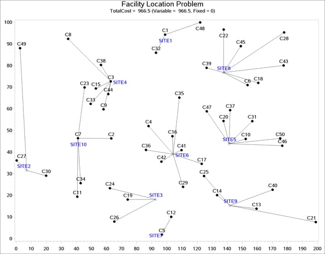
Output 7.3.3: Solution Plot for Facility Location with No Fixed Charges
The output of the second program is shown in Output 7.3.4.
title1 "Facility Location Problem";
title2 "TotalCost = &totalcost (Variable = &varcost, Fixed = &fixcost)";

/* create Annotate data set to draw line between customer and assigned site */
data anno(drop=xi yi xj yj);
   %SYSTEM(2, 2, 2);
   set CostFixedCharge_Data(keep=xi yi xj yj);
   %LINE(xi, yi, xj, yj, *, 1, 1);
run;

proc gplot data=csdata anno=anno;
   axis1 label=none order=(0 to &xmax by 10);
   axis2 label=none order=(0 to &ymax by 10);
   symbol1 value=dot interpol=none
      pointlabel=("#name" nodropcollisions height=1) cv=black;
   symbol2 value=diamond interpol=none
      pointlabel=("#name" nodropcollisions color=blue height=1) cv=blue;
   plot cy*x sy*x / overlay haxis=axis1 vaxis=axis2;
run;
quit;
Output 7.3.4: Solution Plot for Facility Location with Fixed Charges
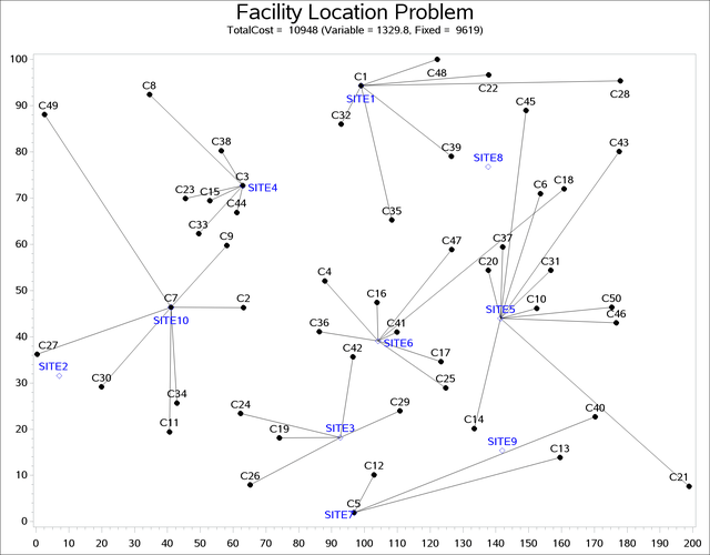
The economic trade-off for the fixed-charge model forces you to build fewer sites and push more demand to each site.
It is possible to expedite the solution of the fixed-charge facility location problem by choosing appropriate branching priorities
for the decision variables. Recall that for each site j, the value of the variable ![]() determines whether or not a facility is built on that site. Suppose you decide to branch on the variables
determines whether or not a facility is built on that site. Suppose you decide to branch on the variables ![]() before the variables
before the variables ![]() . You can set a higher branching priority for
. You can set a higher branching priority for ![]() by using the
by using the .priority suffix for the Build variables in PROC OPTMODEL, as follows:
for{j in SITES} Build[j].priority=10;
Setting higher branching priorities for certain variables is not guaranteed to speed up the MILP solver, but it can be helpful
in some instances. The following program creates and solves an instance of the facility location problem, giving higher priority
to the variables ![]() . The LOGFREQ= option is used to abbreviate the node log.
. The LOGFREQ= option is used to abbreviate the node log.
%let NumCustomers  = 45;
%let NumSites      = 8;
%let SiteCapacity  = 35;
%let MaxDemand     = 10;
%let xmax          = 200;
%let ymax          = 100;
%let seed          = 2345;

/* generate random customer locations */
data cdata(drop=i);
   length name $8;
   do i = 1 to &NumCustomers;
      name = compress('C'||put(i,best.));
      x = ranuni(&seed) * &xmax;
      y = ranuni(&seed) * &ymax;
      demand = ranuni(&seed) * &MaxDemand;
      output;
   end;
run;

/* generate random site locations and fixed charge */
data sdata(drop=i);
length name $8;
   do i = 1 to &NumSites;
      name = compress('SITE'||put(i,best.));
      x = ranuni(&seed) * &xmax;
      y = ranuni(&seed) * &ymax;
      fixed_charge = (abs(&xmax/2-x) + abs(&ymax/2-y)) / 2;
      output;
   end;
run;
proc optmodel;
   set <str> CUSTOMERS;
   set <str> SITES init {};

   /* x and y coordinates of CUSTOMERS and SITES */
   num x {CUSTOMERS union SITES};
   num y {CUSTOMERS union SITES};
   num demand {CUSTOMERS};
   num fixed_charge {SITES};

   /* distance from customer i to site j */
   num dist {i in CUSTOMERS, j in SITES}
       = sqrt((x[i] - x[j])^2 + (y[i] - y[j])^2);

   read data cdata into CUSTOMERS=[name] x y demand;
   read data sdata into SITES=[name] x y fixed_charge;

   var Assign {CUSTOMERS, SITES} binary;
   var Build {SITES} binary;

   min CostFixedCharge
       = sum {i in CUSTOMERS, j in SITES} dist[i,j] * Assign[i,j]
         + sum {j in SITES} fixed_charge[j] * Build[j];

   /* each customer assigned to exactly one site */
   con assign_def {i in CUSTOMERS}:
      sum {j in SITES} Assign[i,j] = 1;

   /* if customer i assigned to site j, then facility must be built at j */
   con link {i in CUSTOMERS, j in SITES}:
      Assign[i,j] <= Build[j];

   /* each site can handle at most &SiteCapacity demand */
   con capacity {j in SITES}:
      sum {i in CUSTOMERS} demand[i] * Assign[i,j] <= &SiteCapacity * Build[j];

   /* assign priority to Build variables (y) */
   for{j in SITES} Build[j].priority=10;

   /* solve the MILP with fixed charges, using branching priorities */
   solve obj CostFixedCharge with milp / logfreq=1000;
quit;
The resulting output is shown in Output 7.3.5.
Output 7.3.5: PROC OPTMODEL Log for Facility Location with Branching Priorities
| Facility Location Problem |
| TotalCost = 10948 (Variable = 1329.8, Fixed = 9619) |
| NOTE: There were 45 observations read from the data set WORK.CDATA. |
| NOTE: There were 8 observations read from the data set WORK.SDATA. |
| NOTE: Problem generation will use 2 threads. |
| NOTE: The problem has 368 variables (0 free, 0 fixed). |
| NOTE: The problem has 368 binary and 0 integer variables. |
| NOTE: The problem has 413 linear constraints (368 LE, 45 EQ, 0 GE, 0 range). |
| NOTE: The problem has 1448 linear constraint coefficients. |
| NOTE: The problem has 0 nonlinear constraints (0 LE, 0 EQ, 0 GE, 0 range). |
| NOTE: The MILP presolver value AUTOMATIC is applied. |
| NOTE: The MILP presolver removed 0 variables and 0 constraints. |
| NOTE: The MILP presolver removed 0 constraint coefficients. |
| NOTE: The MILP presolver modified 0 constraint coefficients. |
| NOTE: The presolved problem has 368 variables, 413 constraints, and 1448 |
| constraint coefficients. |
| NOTE: The MILP solver is called. |
| Node Active Sols BestInteger BestBound Gap Time |
| 0 1 3 2823.1827978 0 2823.2 0 |
| 0 1 3 2823.1827978 1727.0208789 63.47% 0 |
| 0 1 3 2823.1827978 1758.4959444 60.55% 0 |
| 0 1 3 2823.1827978 1777.9581456 58.79% 0 |
| 0 1 3 2823.1827978 1786.2487641 58.05% 0 |
| 0 1 3 2823.1827978 1789.8831106 57.73% 0 |
| 0 1 3 2823.1827978 1791.4930241 57.59% 0 |
| 0 1 3 2823.1827978 1793.9911665 57.37% 0 |
| 0 1 3 2823.1827978 1795.5152566 57.24% 0 |
| 0 1 3 2823.1827978 1796.6395103 57.14% 0 |
| 0 1 3 2823.1827978 1797.2196277 57.09% 0 |
| 0 1 3 2823.1827978 1798.7116308 56.96% 0 |
| 0 1 6 1867.2953460 1799.1463919 3.79% 0 |
| 0 1 6 1867.2953460 1799.4020954 3.77% 0 |
| 0 1 6 1867.2953460 1799.9500748 3.74% 0 |
| 0 1 6 1867.2953460 1800.1075050 3.73% 0 |
| 0 1 6 1867.2953460 1800.1075050 3.73% 0 |
| NOTE: The MILP solver added 32 cuts with 1013 cut coefficients at the root. |
| 16 16 7 1841.9436945 1801.7219901 2.23% 0 |
| 148 136 8 1831.7800505 1805.5957623 1.45% 1 |
| 238 191 9 1826.0904114 1806.4101894 1.09% 1 |
| 307 208 10 1822.8640269 1808.3177036 0.80% 1 |
| 329 203 11 1821.5277612 1808.7906394 0.70% 1 |
| 503 183 12 1821.5115362 1814.4176969 0.39% 2 |
| 604 74 13 1819.9124340 1817.9289922 0.11% 2 |
| 672 9 13 1819.9124340 1819.7313148 0.01% 2 |
| NOTE: Optimal within relative gap. |
| NOTE: Objective = 1819.91243. |