The OPTQP Procedure

Example 12.1 Linear Least Squares Problem

The linear least squares problem arises in the context of determining a solution to an overdetermined set of linear equations. In practice, these equations could arise in data fitting and estimation problems. An overdetermined system of linear equations can be defined as

$\text{[math]}$

where $\text{[math]}$ , $\text{[math]}$ , $\text{[math]}$ , and $\text{[math]}$ . Since this system usually does not have a solution, you need to be satisfied with some sort of approximate solution. The most widely used approximation is the least squares solution, which minimizes $\text{[math]}$ .

This problem is called a least squares problem for the following reason. Let $\text{[math]}$ , $\text{[math]}$ , and $\text{[math]}$ be defined as previously. Let $\text{[math]}$ be the $\text{[math]}$ th component of the vector $\text{[math]}$ :

$\text{[math]}$

By definition of the Euclidean norm, the objective function can be expressed as follows:

$\text{[math]}$

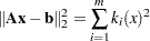Therefore, the function you minimize is the sum of squares of $\text{[math]}$ terms $\text{[math]}$ ; hence the term least squares. The following example is an illustration of the linear least squares problem; that is, each of the terms $\text{[math]}$ is a linear function of $\text{[math]}$ .

Consider the following least squares problem defined by

$\text{[math]}$

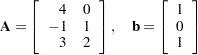This translates to the following set of linear equations:

$\text{[math]}$

The corresponding least squares problem is

$\text{[math]}$

The preceding objective function can be expanded to

$\text{[math]}$

In addition, you impose the following constraint so that the equation $\text{[math]}$ is satisfied within a tolerance of $\text{[math]}$ :

$\text{[math]}$

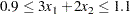You can create the QPS-format input data set by using the following SAS statements:

data lsdata;
   input field1 $ field2 $ field3$ field4 field5 $ field6 @;
datalines;
NAME   .      LEASTSQ     .            .         .
ROWS   .      .           .            .         .
N      OBJ    .           .            .         .
G      EQ3    .           .            .         .
COLUMNS .     .           .            .         .
.      X1     OBJ       -14            EQ3       3
.      X2     OBJ        -4            EQ3       2
RHS    .      .           .            .         .
.      RHS    OBJ        -2            EQ3     0.9
RANGES .      .           .            .         .
.      RNG    EQ3       0.2            .         .
BOUNDS .      .           .            .         .
FR    BND1    X1          .            .         .
FR    BND1    X2          .            .         .
QUADOBJ .     .           .            .         .
.      X1     X1         52            .         .
.      X1     X2         10            .         .
.      X2     X2         10            .         .
ENDATA .      .           .            .         .
;

The decision variables $\text{[math]}$ and $\text{[math]}$ are free, so they have bound type FR in the BOUNDS section of the QPS-format data set.

You can use the following SAS statements to solve the least squares problem:

proc optqp data=lsdata 
   printlevel = 0
   primalout = lspout; 
run;

The optimal solution is displayed in Output 12.1.1.

Output 12.1.1 Solution to the Least Squares Problem

Primal Solution

Obs	Objective Function ID	RHS ID	Variable Name	Variable Type	Linear Objective Coefficient	Lower Bound	Upper Bound	Variable Value	Variable Status
1	OBJ	RHS	X1	F	-14	-1.7977E308	1.7977E308	0.23810	O
2	OBJ	RHS	X2	F	-4	-1.7977E308	1.7977E308	0.16190	O

The iteration log is shown in Output 12.1.2.

Output 12.1.2 Iteration Log

NOTE: The problem LEASTSQ has 2 variables (2 free, 0 fixed).

NOTE: The problem has 1 constraints (0 LE, 0 EQ, 0 GE, 1 range).

NOTE: The problem has 2 constraint coefficients.

NOTE: The objective function has 2 Hessian diagonal elements and 1 Hessian

elements above the diagonal.

NOTE: The OPTQP presolver value AUTOMATIC is applied.

NOTE: The OPTQP presolver removed 0 variables and 0 constraints.

NOTE: The OPTQP presolver removed 0 constraint coefficients.

NOTE: The QUADRATIC ITERATIVE solver is called.

Primal Bound Dual

Iter Complement Duality Gap Infeas Infeas Infeas

0 0.043562 0.007222 1.9636742E-8 0.117851 0.001324

1 0.005868 0.001940 1.97061E-10 0.001179 0.000013242

2 0.000200 0.000066706 5.200219E-12 0.000024662 0.000000277

3 0.000002080 0.000000695 1.718896E-13 0.000000248 2.7859102E-9

4 0 7.425058E-17 0 0 3.940437E-17

NOTE: Optimal.

NOTE: Objective = 0.00952380952.

NOTE: The data set WORK.LSPOUT has 2 observations and 9 variables.