The Mixed Integer Linear Programming Solver

Example 6.3 Facility Location
Consider the classic facility location problem. Given a set  of customer locations and a set
  of candidate facility sites, you must decide on which sites to build facilities and assign coverage of customer demand to these sites so as to minimize cost. All customer demand
  must be satisfied, and each facility has a demand capacity limit
  . The total cost is the sum of the distances
  between facility
  and its assigned customer
  , plus a fixed charge
  for building a facility at site . Let
  represent choosing site to build a facility, and 0 otherwise. Also, let
  represent the assignment of customer to facility , and 0 otherwise. This model can be formulated as the following integer linear program:
 |
Constraint (assign_def) ensures that each customer is assigned to exactly one site. Constraint (link) forces a facility to be built if any customer has been assigned to that facility. Finally, constraint (capacity) enforces the capacity limit at each site.
Consider also a variation of this same problem where there is no cost for building a facility. This problem is typically easier to solve than the original problem. For this variant, let the objective be
 |
First, construct a random instance of this problem by using the following DATA steps:
title 'Facility Location Problem';
%let NumCustomers  = 50;
%let NumSites      = 10;
%let SiteCapacity  = 35;
%let MaxDemand     = 10;
%let xmax          = 200;
%let ymax          = 100;
%let seed          = 938;

/* generate random customer locations */
data cdata(drop=i);
   length name $8;
   do i = 1 to &NumCustomers;
      name = compress('C'||put(i,best.));
      x = ranuni(&seed) * &xmax;
      y = ranuni(&seed) * &ymax;
      demand = ranuni(&seed) * &MaxDemand;
      output;
   end;
run;

/* generate random site locations and fixed charge */
data sdata(drop=i);
   length name $8;
   do i = 1 to &NumSites;
      name = compress('SITE'||put(i,best.));
      x = ranuni(&seed) * &xmax;
      y = ranuni(&seed) * &ymax;
      fixed_charge = 30 * (abs(&xmax/2-x) + abs(&ymax/2-y));
      output;
   end;
run;
The following PROC OPTMODEL statements first generate and solve the model with the no-fixed-charge variant of the cost function. Next, they solve the fixed-charge model. Note that the solution to the model with no fixed charge is feasible for the fixed-charge model and should provide a good starting point for the MILP solver. Use the PRIMALIN option to provide an incumbent solution (warm start).
proc optmodel;
    set <str> CUSTOMERS;
    set <str> SITES init {};

    /* x and y coordinates of CUSTOMERS and SITES */
    num x {CUSTOMERS union SITES};
    num y {CUSTOMERS union SITES};
    num demand {CUSTOMERS};
    num fixed_charge {SITES};

    /* distance from customer i to site j */
    num dist {i in CUSTOMERS, j in SITES}
        = sqrt((x[i] - x[j])^2 + (y[i] - y[j])^2);

    read data cdata into CUSTOMERS=[name] x y demand;
    read data sdata into SITES=[name] x y fixed_charge;

    var Assign {CUSTOMERS, SITES} binary;
    var Build {SITES} binary;

    min CostNoFixedCharge
        = sum {i in CUSTOMERS, j in SITES} dist[i,j] * Assign[i,j];
    min CostFixedCharge
        = CostNoFixedCharge + sum {j in SITES} fixed_charge[j] * Build[j];

    /* each customer assigned to exactly one site */
    con assign_def {i in CUSTOMERS}:
       sum {j in SITES} Assign[i,j] = 1;

    /* if customer i assigned to site j, then facility must be built at j */
    con link {i in CUSTOMERS, j in SITES}:
        Assign[i,j] <= Build[j];

    /* each site can handle at most &SiteCapacity demand */
    con capacity {j in SITES}:
        sum {i in CUSTOMERS} demand[i] * Assign[i,j] <=
            &SiteCapacity * Build[j];

    /* solve the MILP with no fixed charges */
    solve obj CostNoFixedCharge with milp / printfreq = 500;

    /* clean up the solution */
    for {i in CUSTOMERS, j in SITES} Assign[i,j] = round(Assign[i,j]);
    for {j in SITES} Build[j] = round(Build[j]);

    call symput('varcostNo',put(CostNoFixedCharge,6.1));

    /* create a data set for use by GPLOT */
    create data CostNoFixedCharge_Data from
        [customer site]={i in CUSTOMERS, j in SITES: Assign[i,j] = 1}
        xi=x[i] yi=y[i] xj=x[j] yj=y[j];
    /* solve the MILP, with fixed charges with warm start */
    solve obj CostFixedCharge with milp / primalin printfreq = 500;

    /* clean up the solution */
    for {i in CUSTOMERS, j in SITES} Assign[i,j] = round(Assign[i,j]);
    for {j in SITES} Build[j] = round(Build[j]);

    num varcost = sum {i in CUSTOMERS, j in SITES} dist[i,j] * Assign[i,j].sol;
    num fixcost = sum {j in SITES} fixed_charge[j] * Build[j].sol;
    call symput('varcost', put(varcost,6.1));
    call symput('fixcost', put(fixcost,5.1));
    call symput('totalcost', put(CostFixedCharge,6.1));

    /* create a data set for use by GPLOT */
    create data CostFixedCharge_Data from
        [customer site]={i in CUSTOMERS, j in SITES: Assign[i,j] = 1}
        xi=x[i] yi=y[i] xj=x[j] yj=y[j];
 quit;
The information printed in the log for the no-fixed-charge model is displayed in Output 6.3.1.
| Facility Location Problem |
| NOTE: The problem has 510 variables (0 free, 0 fixed). |
| NOTE: The problem has 510 binary and 0 integer variables. |
| NOTE: The problem has 560 linear constraints (510 LE, 50 EQ, 0 GE, 0 range). |
| NOTE: The problem has 2010 linear constraint coefficients. |
| NOTE: The problem has 0 nonlinear constraints (0 LE, 0 EQ, 0 GE, 0 range). |
| NOTE: The OPTMILP presolver value AUTOMATIC is applied. |
| NOTE: The OPTMILP presolver removed 10 variables and 500 constraints. |
| NOTE: The OPTMILP presolver removed 1010 constraint coefficients. |
| NOTE: The OPTMILP presolver modified 0 constraint coefficients. |
| NOTE: The presolved problem has 500 variables, 60 constraints, and 1000 |
| constraint coefficients. |
| NOTE: The MIXED INTEGER LINEAR solver is called. |
| Node Active Sols BestInteger BestBound Gap Time |
| 0 1 2 972.1737321 0 972.2 0 |
| 0 1 2 972.1737321 961.2403449 1.14% 0 |
| 0 1 3 966.4832160 966.4832160 0.00% 0 |
| 0 0 3 966.4832160 . 0.00% 0 |
| NOTE: OPTMILP added 6 cuts with 360 cut coefficients at the root. |
| NOTE: Optimal. |
| NOTE: Objective = 966.483216. |
The results from the warm start approach are shown in Output 6.3.2.
| Facility Location Problem |
| NOTE: The problem has 510 variables (0 free, 0 fixed). |
| NOTE: The problem uses 1 implicit variables. |
| NOTE: The problem has 510 binary and 0 integer variables. |
| NOTE: The problem has 560 linear constraints (510 LE, 50 EQ, 0 GE, 0 range). |
| NOTE: The problem has 2010 linear constraint coefficients. |
| NOTE: The problem has 0 nonlinear constraints (0 LE, 0 EQ, 0 GE, 0 range). |
| NOTE: The OPTMILP presolver value AUTOMATIC is applied. |
| NOTE: The OPTMILP presolver removed 0 variables and 0 constraints. |
| NOTE: The OPTMILP presolver removed 0 constraint coefficients. |
| NOTE: The OPTMILP presolver modified 0 constraint coefficients. |
| NOTE: The presolved problem has 510 variables, 560 constraints, and 2010 |
| constraint coefficients. |
| NOTE: The MIXED INTEGER LINEAR solver is called. |
| Node Active Sols BestInteger BestBound Gap Time |
| 0 1 3 16070.0150023 0 16070 0 |
| 0 1 3 16070.0150023 9946.2514269 61.57% 0 |
| 0 1 3 16070.0150023 10930.3459381 47.02% 0 |
| 0 1 3 16070.0150023 10935.7635056 46.95% 0 |
| 0 1 3 16070.0150023 10937.6002156 46.92% 0 |
| 0 1 3 16070.0150023 10940.1196005 46.89% 0 |
| 0 1 6 12678.8372466 10940.5372019 15.89% 0 |
| 0 1 7 10971.6925169 10940.5372019 0.28% 0 |
| NOTE: OPTMILP added 15 cuts with 463 cut coefficients at the root. |
| 2 3 8 10970.7775646 10941.8374374 0.26% 0 |
| 9 10 9 10948.4603381 10941.8374374 0.06% 0 |
| 10 10 10 10948.4603380 10941.8374374 0.06% 0 |
| 30 0 10 10948.4603380 . 0.00% 1 |
| NOTE: Optimal. |
| NOTE: Objective = 10948.4603. |
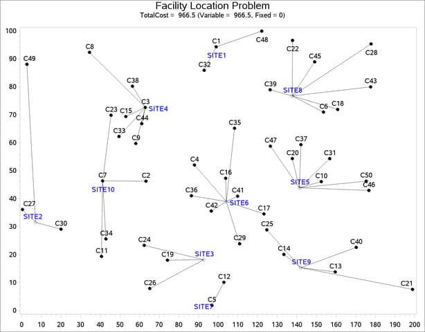
The following two SAS programs produce a plot of the solutions for both variants of the model, using data sets produced by PROC OPTMODEL:
title1 h=1.5 "Facility Location Problem";
title2 "TotalCost = &varcostNo (Variable = &varcostNo, Fixed = 0)";
data csdata;
    set cdata(rename=(y=cy)) sdata(rename=(y=sy));
run;
/* create Annotate data set to draw line between customer and assigned site */
%annomac;
data anno(drop=xi yi xj yj);
   %SYSTEM(2, 2, 2);
   set CostNoFixedCharge_Data(keep=xi yi xj yj);
   %LINE(xi, yi, xj, yj, *, 1, 1);
run;
proc gplot data=csdata anno=anno;
   axis1 label=none order=(0 to &xmax by 10);
   axis2 label=none order=(0 to &ymax by 10);
   symbol1 value=dot interpol=none
      pointlabel=("#name" nodropcollisions height=1) cv=black;
   symbol2 value=diamond interpol=none
      pointlabel=("#name" nodropcollisions color=blue height=1) cv=blue;
   plot cy*x sy*x / overlay haxis=axis1 vaxis=axis2;
run;
quit;
The output of the first program is shown in Output 6.3.3.
The output of the second program is shown in Output 6.3.4.
title1 "Facility Location Problem";
title2 "TotalCost = &totalcost (Variable = &varcost, Fixed = &fixcost)";
/* create Annotate data set to draw line between customer and assigned site */
data anno(drop=xi yi xj yj);
   %SYSTEM(2, 2, 2);
   set CostFixedCharge_Data(keep=xi yi xj yj);
   %LINE(xi, yi, xj, yj, *, 1, 1);
run;
proc gplot data=csdata anno=anno;
   axis1 label=none order=(0 to &xmax by 10);
   axis2 label=none order=(0 to &ymax by 10);
   symbol1 value=dot interpol=none
      pointlabel=("#name" nodropcollisions height=1) cv=black;
   symbol2 value=diamond interpol=none
      pointlabel=("#name" nodropcollisions color=blue height=1) cv=blue;
   plot cy*x sy*x / overlay haxis=axis1 vaxis=axis2;
run;
quit;
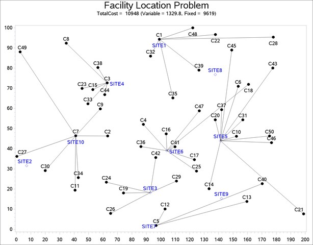
The economic trade-off for the fixed-charge model forces you to build fewer sites and push more demand to each site.
It is possible to expedite the solution of the fixed-charge facility location problem by choosing appropriate branching priorities for the decision variables. Recall that for each site , the value of the variable  determines whether or not a facility is built on that site. Suppose you decide to branch on the variables before the variables
  . You can set a higher branching priority for by using the .priority suffix for the Build variables in PROC OPTMODEL, as follows:
for{j in SITES} Build[j].priority=10;
Setting higher branching priorities for certain variables is not guaranteed to speed up the MILP solver, but it can be helpful in some instances. The following program creates and solves an instance of the facility location problem, giving higher priority to the variables . The PRINTFREQ= option is used to abbreviate the node log.
    %let NumCustomers  = 45;
    %let NumSites      = 8;
    %let SiteCapacity  = 35;
    %let MaxDemand     = 10;
    %let xmax          = 200;
    %let ymax          = 100;
    %let seed          = 2345;

    /* generate random customer locations */
    data cdata(drop=i);
       length name $8;
       do i = 1 to &NumCustomers;
          name = compress('C'||put(i,best.));
          x = ranuni(&seed) * &xmax;
          y = ranuni(&seed) * &ymax;
          demand = ranuni(&seed) * &MaxDemand;
          output;
       end;
    run;

    /* generate random site locations and fixed charge */
    data sdata(drop=i);
       length name $8;
       do i = 1 to &NumSites;
          name = compress('SITE'||put(i,best.));
          x = ranuni(&seed) * &xmax;
          y = ranuni(&seed) * &ymax;
          fixed_charge = (abs(&xmax/2-x) + abs(&ymax/2-y)) / 2;
          output;
       end;
    run;
proc optmodel;
   set <str> CUSTOMERS;
   set <str> SITES init {};
   /* x and y coordinates of CUSTOMERS and SITES */
   num x {CUSTOMERS union SITES};
   num y {CUSTOMERS union SITES};
   num demand {CUSTOMERS};
   num fixed_charge {SITES};

   /* distance from customer i to site j */
   num dist {i in CUSTOMERS, j in SITES}
       = sqrt((x[i] - x[j])^2 + (y[i] - y[j])^2);
   read data cdata into CUSTOMERS=[name] x y demand;
   read data sdata into SITES=[name] x y fixed_charge;
   var Assign {CUSTOMERS, SITES} binary;
   var Build {SITES} binary;
   min CostFixedCharge
       = sum {i in CUSTOMERS, j in SITES} dist[i,j] * Assign[i,j]
         + sum {j in SITES} fixed_charge[j] * Build[j];

   /* each customer assigned to exactly one site */
   con assign_def {i in CUSTOMERS}:
      sum {j in SITES} Assign[i,j] = 1;
   /* if customer i assigned to site j, then facility must be built at j */
   con link {i in CUSTOMERS, j in SITES}:
       Assign[i,j] <= Build[j];
   /* each site can handle at most &SiteCapacity demand */
   con capacity {j in SITES}:
       sum {i in CUSTOMERS} demand[i] * Assign[i,j] <= &SiteCapacity * Build[j];
   /* assign priority to Build variables (y) */
   for{j in SITES} Build[j].priority=10;
   /* solve the MILP with fixed charges, using branching priorities */
   solve obj CostFixedCharge with milp / printfreq=1000;

quit;
The resulting output is shown in Output 6.3.5.
| Facility Location Problem |
| TotalCost = 10948 (Variable = 1329.8, Fixed = 9619) |
| NOTE: There were 45 observations read from the data set WORK.CDATA. |
| NOTE: There were 8 observations read from the data set WORK.SDATA. |
| NOTE: The problem has 368 variables (0 free, 0 fixed). |
| NOTE: The problem has 368 binary and 0 integer variables. |
| NOTE: The problem has 413 linear constraints (368 LE, 45 EQ, 0 GE, 0 range). |
| NOTE: The problem has 1448 linear constraint coefficients. |
| NOTE: The problem has 0 nonlinear constraints (0 LE, 0 EQ, 0 GE, 0 range). |
| NOTE: The OPTMILP presolver value AUTOMATIC is applied. |
| NOTE: The OPTMILP presolver removed 0 variables and 0 constraints. |
| NOTE: The OPTMILP presolver removed 0 constraint coefficients. |
| NOTE: The OPTMILP presolver modified 0 constraint coefficients. |
| NOTE: The presolved problem has 368 variables, 413 constraints, and 1448 |
| constraint coefficients. |
| NOTE: The MIXED INTEGER LINEAR solver is called. |
| Node Active Sols BestInteger BestBound Gap Time |
| 0 1 3 2823.1827978 0 2823.2 0 |
| 0 1 3 2823.1827978 1727.0208789 63.47% 0 |
| 0 1 3 2823.1827978 1763.3506901 60.10% 0 |
| 0 1 3 2823.1827978 1777.2135752 58.85% 0 |
| 0 1 3 2823.1827978 1784.9548182 58.17% 0 |
| 0 1 3 2823.1827978 1787.1819351 57.97% 0 |
| 0 1 3 2823.1827978 1793.2692707 57.43% 0 |
| 0 1 3 2823.1827978 1794.3938422 57.33% 0 |
| 0 1 3 2823.1827978 1795.3899713 57.25% 0 |
| 0 1 3 2823.1827978 1798.5234862 56.97% 0 |
| 0 1 3 2823.1827978 1799.5894342 56.88% 0 |
| 0 1 3 2823.1827978 1800.5233791 56.80% 0 |
| 0 1 3 2823.1827978 1800.6378795 56.79% 0 |
| 0 1 3 2823.1827978 1800.7748861 56.78% 0 |
| 0 1 5 1842.4563183 1801.0525162 2.30% 0 |
| 0 1 5 1842.4563183 1801.5520700 2.27% 0 |
| NOTE: OPTMILP added 31 cuts with 851 cut coefficients at the root. |
| 107 103 7 1839.8099830 1802.5501263 2.07% 0 |
| 256 227 8 1835.4822150 1804.7295110 1.70% 1 |
| 257 207 9 1825.1665993 1804.7295110 1.13% 1 |
| 344 255 10 1823.4483964 1805.3755931 1.00% 1 |
| 380 281 11 1823.3287598 1805.7995246 0.97% 1 |
| 503 260 12 1819.9124350 1809.1789223 0.59% 1 |
| 752 125 13 1819.9124339 1815.3056997 0.25% 2 |
| 890 4 13 1819.9124339 1819.7542550 0.01% 2 |
| NOTE: Optimal within relative gap. |
| NOTE: Objective = 1819.91243. |