Previous Page

|

Next Page

The Sequential Quadratic Programming Solver

Getting Started: SQP Solver

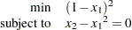
Consider a simple example of minimizing the following nonlinear programming problem:

Assume the starting point 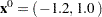. You can use the following SAS code to solve the problem:

proc optmodel;
  var x {1..2};
  minimize obj = (1-x[1])^2;

  con cons1: x[2] - x[1]^2 = 0;

  /*starting point */
  x[1] = -1.2;
  x[2] =  1;

  solve with SQP/ printfreq = 5;
  print x;

quit;   

The summary of the solver output along with the optimal solution, , is displayed in Figure 15.1.

Figure 15.1 Optimal Solution

The OPTMODEL Procedure

Problem Summary
Objective Sense	Minimization
Objective Function	obj
Objective Type	Quadratic
Number of Variables	2
Bounded Above	0
Bounded Below	0
Bounded Below and Above	0
Free	2
Fixed	0
Number of Constraints	1
Linear LE (<=)	0
Linear EQ (=)	0
Linear GE (>=)	0
Linear Range	0
Nonlinear LE (<=)	0
Nonlinear EQ (=)	1
Nonlinear GE (>=)	0
Nonlinear Range	0

Solution Summary
Solver	SQP
Objective Function	obj
Solution Status	Optimal
Objective Value	2.652572E-12
Iterations	26
Infeasibility	5.7837896E-7
Optimality Error	2.0208534E-6
Complementarity	0

[1]	x
1	1
2	1

The iteration log in Figure 15.2 displays information about the objective function value, the norm of the violated constraints, the norm of the gradient of the Lagrangian function, and the norm of the violated complementarity condition at each iteration.

Copyright © SAS Institute, Inc. All Rights Reserved.