The OPTMILP Procedure

Getting Started: OPTMILP Procedure

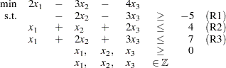
The following example illustrates the use of the OPTMILP procedure to solve mixed integer linear programs. For more examples, see the section Examples: OPTMILP Procedure. Suppose you want to solve the following problem:

$\text{[math]}$

The corresponding MPS-format SAS data set follows:

data ex_mip;   
   input field1 $ field2 $ field3 $ field4 field5 $ field6;
   datalines;
NAME        .      EX_MIP      .   .        .
ROWS        .        .         .   .        .
N           COST     .         .   .        .
G           R1       .         .   .        .
L           R2       .         .   .        .
L           R3       .         .   .        . 
COLUMNS     .        .         .   .        .
.           MARK00 'MARKER'    .   'INTORG' .
.           X1     COST        2   R2       1   
.           X1     R3          1   .        .   
.           X2     COST       -3   R1      -2
.           X2     R2          1   R3       2
.           X3     COST       -4   R1      -3
.           X3     R2          2   R3       3
.           MARK01 'MARKER'    .   'INTEND' .
RHS         .      .           .   .        .
.           RHS    R1         -5   R2       4   
.           RHS    R3          7   .        .
ENDATA      .      .           .   .        .
;

You can also create this SAS data set from an MPS-format flat file (ex_mip.mps) by using the following SAS macro:

   %mps2sasd(mpsfile = "ex_mip.mps", outdata = ex_mip);

This problem can be solved by using the following statement to call the OPTMILP procedure:

proc optmilp data = ex_mip 
   objsense   = min
   primalout  = primal_out 
   dualout    = dual_out
   presolver  = automatic
   heuristics = automatic; 
run;

The DATA= option names the MPS-format SAS data set containing the problem data. The OBJSENSE= option specifies whether to maximize or minimize the objective function. The PRIMALOUT= option names the SAS data set containing the optimal solution or the best feasible solution found by the solver. The DUALOUT= option names the SAS data set containing the constraint activities. The PRESOLVER= and HEURISTICS= options specify the levels for presolving and applying heuristics, respectively. In this example, each option is set to its default value AUTOMATIC, meaning that the solver determines the appropriate levels for presolve and heuristics automatically.

The optimal integer solution and its corresponding constraint activities, stored in the data sets primal_out and dual_out, respectively, are displayed in Figure 18.1 and Figure 18.2.

Figure 18.1 Optimal Solution

The OPTMILP Procedure

Primal Integer Solution

Obs	Objective Function ID	RHS ID	Variable Name	Variable Type	Objective Coefficient	Upper Bound	Variable Value
1	COST	RHS	X1	B	2	1	0
2	COST	RHS	X2	B	-3	1	1
3	COST	RHS	X3	B	-4	1	1

Figure 18.2 Constraint Activities

The OPTMILP Procedure

Constraint Information

Obs	Objective Function ID	RHS ID	Constraint Name	Constraint Type	Constraint RHS	Constraint Lower Bound	Constraint Upper Bound	Constraint Activity
1	COST	RHS	R1	G	-5	.	.	-5
2	COST	RHS	R2	L	4	.	.	3
3	COST	RHS	R3	L	7	.	.	5

The solution summary stored in the macro variable _OROPTMILP_ can be viewed by issuing the following statement:


   %put &_OROPTMILP_;

This produces the output shown in Figure 18.3.

Figure 18.3 Macro Output

The OPTMILP Procedure

Constraint Information


STATUS=OK SOLUTION_STATUS=OPTIMAL OBJECTIVE=-7 RELATIVE_GAP=0
ABSOLUTE_GAP=0 PRIMAL_INFEASIBILITY=0 BOUND_INFEASIBILITY=0
INTEGER_INFEASIBILITY=0 BEST_BOUND=. NODES=0 ITERATIONS=0
PRESOLVE_TIME=0.00 SOLUTION_TIME=0.00

See the section Data Input and Output for details about the type and status codes displayed for variables and constraints.

Top of Page