| The NETFLOW Procedure |
Example 7.14 Generalized Networks: Distribution Problem
Consider a distribution problem (from Jensen and Bard 2003) with three supply plants ( –
–  ) and five demand points (
 –
–  ). Further information about the problem is as follows:
To be closed. Entire inventory must be shipped or sold to scrap. The scrap value is $5 per unit.

Maximum production of 300 units with manufacturing cost of $10 per unit.
The production in regular time amounts to 200 units and must be shipped. An additional 100 units can be produced using overtime at $14 per unit.
Fixed demand of 200 units must be met.

Contracted demand of 300 units. An additional 100 units can be sold at $20 per unit.

Minimum demand of 200 units. An additional 100 units can be sold at $20 per unit. Additional units can be procured from
 at $4 per unit. There is a 5% "shipping loss" on the arc connecting these two nodes.
 Fixed demand of 150 units must be met.
100 units left over from previous shipments. No firm demand, but up to 250 units can be sold at $25 per unit.
Additionally, there is a 5% "shipping loss" on each of the arcs between supply and demand nodes.
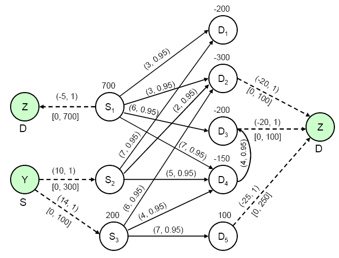
You can model this scenario as a generalized network. Since there are both fixed and varying supply and demand supdem values, you can transform this to a case where you need to address missing supply and demand simultaneously. As seen from Output 7.14.1, we have added two artificial nodes, Y and Z, with missing S supply value and missing D demand value, respectively. The extra production capability is depicted by arcs from node Y to the corresponding supply nodes, and the extra revenue generation capability of the demand points (and scrap revenue for ) is depicted by arcs to node Z.
The following SAS data set has the complete information about the arc costs, multipliers, and node supdem values:
data dnodes;
   input _node_ $ _sd_ ;
   missing S D;
datalines;
S1   700
S2     0
S3   200
D1  -200
D2  -300
D3  -200
D4  -150
D5   100
Y      S
Z      D
;

data darcs;
   input _from_ $ _to_ $ _cost_ _capac_ _mult_;
datalines;
S1  D1    3   200  0.95
S1  D2    3   200  0.95
S1  D3    6   200  0.95
S1  D4    7   200  0.95
S2  D1    7   200  0.95
S2  D2    2   200  0.95
S2  D4    5   200  0.95
S3  D2    6   200  0.95
S3  D4    4   200  0.95
S3  D5    7   200  0.95
D4  D3    4   200  0.95
Y   S2   10   300  .
Y   S3   14   100  .
S1  Z   -5    700  .
D2  Z   -20   100  .
D3  Z   -20   100  .
D5  Z   -25   250  .
;
You can solve this problem by using the following call to PROC NETFLOW:
title1 'The NETFLOW Procedure';
proc netflow
   nodedata = dnodes
   arcdata  = darcs
   conout   = dsol;
run;
The optimal solution is displayed in Output 7.14.2.
| The NETFLOW Procedure |
| Obs | _from_ | _to_ | _cost_ | _capac_ | _LO_ | _mult_ | _SUPPLY_ | _DEMAND_ | _FLOW_ | _FCOST_ |
|---|---|---|---|---|---|---|---|---|---|---|
| 1 | S1 | D1 | 3 | 200 | 0 | 0.95 | 700 | 200 | 200.000 | 600.00 |
| 2 | S2 | D1 | 7 | 200 | 0 | 0.95 | . | 200 | 10.526 | 73.68 |
| 3 | S1 | D2 | 3 | 200 | 0 | 0.95 | 700 | 300 | 200.000 | 600.00 |
| 4 | S2 | D2 | 2 | 200 | 0 | 0.95 | . | 300 | 200.000 | 400.00 |
| 5 | S3 | D2 | 6 | 200 | 0 | 0.95 | 200 | 300 | 21.053 | 126.32 |
| 6 | S1 | D3 | 6 | 200 | 0 | 0.95 | 700 | 200 | 200.000 | 1200.00 |
| 7 | D4 | D3 | 4 | 200 | 0 | 0.95 | . | 200 | 10.526 | 42.11 |
| 8 | S1 | D4 | 7 | 200 | 0 | 0.95 | 700 | 150 | 100.000 | 700.00 |
| 9 | S2 | D4 | 5 | 200 | 0 | 0.95 | . | 150 | 47.922 | 239.61 |
| 10 | S3 | D4 | 4 | 200 | 0 | 0.95 | 200 | 150 | 21.053 | 84.21 |
| 11 | S3 | D5 | 7 | 200 | 0 | 0.95 | 200 | . | 157.895 | 1105.26 |
| 12 | Y | S2 | 10 | 300 | 0 | 1.00 | S | . | 258.449 | 2584.49 |
| 13 | Y | S3 | 14 | 100 | 0 | 1.00 | S | . | 0.000 | 0.00 |
| 14 | S1 | Z | -5 | 700 | 0 | 1.00 | 700 | D | 0.000 | 0.00 |
| 15 | D2 | Z | -20 | 100 | 0 | 1.00 | . | D | 100.000 | -2000.00 |
| 16 | D3 | Z | -20 | 100 | 0 | 1.00 | . | D | 0.000 | 0.00 |
| 17 | D5 | Z | -25 | 250 | 0 | 1.00 | 100 | D | 250.000 | -6250.00 |
| -494.32 |
Copyright © SAS Institute, Inc. All Rights Reserved.