| The Linear Programming Solver |
Getting Started: LP Solver
The following example illustrates how you can use the OPTMODEL procedure to solve linear programs. Suppose you want to solve the following problem:
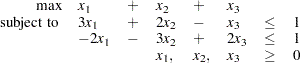 |
You can use the following statement to call the OPTMODEL procedure for solving linear programs:
proc optmodel;
   var x{i in 1..3} >= 0;
   max f = x[1] + x[2] + x[3] ;
   con c1: 3*x[1] + 2*x[2]  - x[3]       <= 1;
   con c2: -2*x[1]  - 3*x[2]  +  2*x[3]  <= 1;
   solve with lp / solver = ps presolver = none printfreq = 1;
   print x;
quit;
The optimal solution and the optimal objective value are displayed in Figure 10.1.
| Problem Summary | |
|---|---|
| Objective Sense | Maximization |
| Objective Function | f |
| Objective Type | Linear |
| Number of Variables | 3 |
| Bounded Above | 0 |
| Bounded Below | 3 |
| Bounded Below and Above | 0 |
| Free | 0 |
| Fixed | 0 |
| Number of Constraints | 2 |
| Linear LE (<=) | 2 |
| Linear EQ (=) | 0 |
| Linear GE (>=) | 0 |
| Linear Range | 0 |
The iteration log displaying problem statistics, progress of the solution, and the optimal objective value is shown in Figure 10.2.
Figure 10.2
Log
| line |
|---|
| NOTE: The problem has 3 variables (0 free, 0 fixed). |
| NOTE: The problem has 2 linear constraints (2 LE, 0 EQ, 0 GE, 0 range). |
| NOTE: The problem has 6 linear constraint coefficients. |
| NOTE: The problem has 0 nonlinear constraints (0 LE, 0 EQ, 0 GE, 0 range). |
| NOTE: The OPTMODEL presolver removed 0 variables, 0 linear constraints, and 0 |
| nonlinear constraints. |
| WARNING: No output destinations active. |
| NOTE: The OPTLP presolver value NONE is applied. |
| NOTE: The PRIMAL SIMPLEX solver is called. |
| Objective Entering Leaving |
| Phase Iteration Value Variable Variable |
| 2 1 0.500000 x[3] c2 (S) |
| 2 2 8.000000 x[2] c1 (S) |
| NOTE: Optimal. |
| NOTE: Objective = 8. |
Copyright © SAS Institute, Inc. All Rights Reserved.