| Introduction to Optimization |
Exploiting Model Structure
Another example helps to illustrate how the model can be simplified by exploiting the structure in the model when using the NETFLOW procedure.
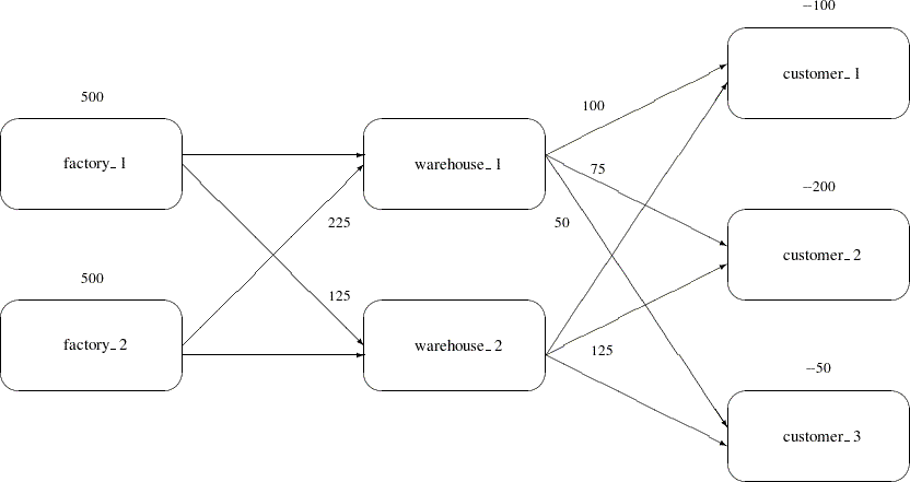
Recall the chocolate transshipment problem discussed previously. The solution required no production at factory_1 and no storage at warehouse_2. Suppose this solution, although optimal, is unacceptable. An additional constraint requiring the production at the two factories to be balanced is needed. Now, the production at the two factories can differ by, at most, 100 units. Such a constraint might look like this:
   -100 <= (factory_1_warehouse_1 + factory_1_warehouse_2 -
            factory_2_warehouse_1 - factory_2_warehouse_2) <= 100
The network and supply and demand information are saved in the following two data sets:
data network;
   format from $12. to $12.;
   input  from $ to $ cost ;
   datalines;
factory_1    warehouse_1  10
factory_2    warehouse_1   5
factory_1    warehouse_2   7
factory_2    warehouse_2   9
warehouse_1  customer_1   3
warehouse_1  customer_2   4
warehouse_1  customer_3   4
warehouse_2  customer_1   5
warehouse_2  customer_2   5
warehouse_2  customer_3   6
;

data nodes;
   format node $12. ;
   input node $  supdem;
   datalines;
customer_1   -100
customer_2   -200
customer_3    -50
factory_1     500
factory_2     500
;
The factory-balancing constraint is not a part of the network. It is represented in the sparse format in a data set for side constraints.
data side_con;
   format _type_ $8. _row_ $8. _col_ $21. ;
   input  _type_  _row_  _col_  _coef_ ;
   datalines;
eq       balance   .                         .
.        balance  factory_1_warehouse_1      1
.        balance  factory_1_warehouse_2      1
.        balance  factory_2_warehouse_1     -1
.        balance  factory_2_warehouse_2     -1
.        balance  diff                      -1
lo       lowerbd  diff                    -100
up       upperbd  diff                     100
;
This data set contains an equality constraint that sets the value of DIFF to be the amount that factory 1 production exceeds factory 2 production. It also contains implicit bounds on the DIFF variable. Note that the DIFF variable is a nonarc variable.
You can use the following call to PROC NETFLOW to solve the problem:
proc netflow
   conout=con_sav
   arcdata=network nodedata=nodes condata=side_con
   sparsecondata ;
   node node;
   supdem supdem;
   tail from;
   head to;
   cost cost;
   run;

proc print;
   var from to _name_ cost _capac_ _lo_ _supply_ _demand_
       _flow_ _fcost_ _rcost_;
   sum _fcost_;
   run;
The solution is saved in the con_sav data set, as displayed in Figure 3.7.
| Obs | from | to | _NAME_ | cost | _CAPAC_ | _LO_ | _SUPPLY_ | _DEMAND_ | _FLOW_ | _FCOST_ | _RCOST_ |
|---|---|---|---|---|---|---|---|---|---|---|---|
| 1 | warehouse_1 | customer_1 | 3 | 99999999 | 0 | . | 100 | 100 | 300 | . | |
| 2 | warehouse_2 | customer_1 | 5 | 99999999 | 0 | . | 100 | 0 | 0 | 1.0 | |
| 3 | warehouse_1 | customer_2 | 4 | 99999999 | 0 | . | 200 | 75 | 300 | . | |
| 4 | warehouse_2 | customer_2 | 5 | 99999999 | 0 | . | 200 | 125 | 625 | . | |
| 5 | warehouse_1 | customer_3 | 4 | 99999999 | 0 | . | 50 | 50 | 200 | . | |
| 6 | warehouse_2 | customer_3 | 6 | 99999999 | 0 | . | 50 | 0 | 0 | 1.0 | |
| 7 | factory_1 | warehouse_1 | 10 | 99999999 | 0 | 500 | . | 0 | 0 | 2.0 | |
| 8 | factory_2 | warehouse_1 | 5 | 99999999 | 0 | 500 | . | 225 | 1125 | . | |
| 9 | factory_1 | warehouse_2 | 7 | 99999999 | 0 | 500 | . | 125 | 875 | . | |
| 10 | factory_2 | warehouse_2 | 9 | 99999999 | 0 | 500 | . | 0 | 0 | 5.0 | |
| 11 | diff | 0 | 100 | -100 | . | . | -100 | 0 | 1.5 | ||
| 3425 |
Notice that the solution now has production balanced across the factories; the production at factory 2 exceeds that at factory 1 by 100 units.
Copyright © SAS Institute, Inc. All Rights Reserved.