| The Quadratic Programming Solver -- Experimental |
Example 12.1: Linear Least-Squares Problem
The linear least-squares problem arises in the context of determining a solution to an over-determined set of linear equations. In practice, these could arise in data fitting and estimation problems. An over-determined system of linear equations can be defined as
This problem is called a least-squares problem for the following reason. Let ![]() ,
, ![]() , and
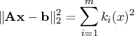
, and ![]() be defined as previously. Let
be defined as previously. Let ![]() be the
be the ![]() th component of the vector
th component of the vector ![]() :
:
![\mathbf{a} = [4 & 0 \ -1 & 1 \ 3 & 2 ], \mathbf{b} = [1 \ 0 \ 1 ]](images/qpsolver_qpsolvereq83.gif)
You can use the following SAS code to solve the least-squares problem:
    /* example 1: linear least-squares problem */
    proc optmodel;
       var x1; /* declare free (no explicit bounds) variable x1 */
       var x2; /* declare free (no explicit bounds) variable x2 */
       /* declare slack variable for ranged constraint */
       var w >= 0 <= 0.2;

       /* objective function: minimize is the sum of squares */
       minimize f = 26 * x1 * x1 + 5 * x2 * x2 + 10 * x1 * x2
           - 14 * x1 - 4 * x2 + 2;

       /* subject to the following constraint */
       con L: 3 * x1 + 2 * x2 - w = 0.9;

       solve with qp;

       /* print the optimal solution */
       print x1 x2;
    quit;
The output is shown in Output 12.1.1.
Output 12.1.1: Summaries and Optimal Solution
Copyright © 2008 by SAS Institute Inc., Cary, NC, USA. All rights reserved.