PROC OPTMODEL: Dual Values :: SAS/OR(R) 9.2 User's Guide: Mathematical Programming

The OPTMODEL Procedure

Dual Values

A dual value is associated with each constraint. To access the dual value of a constraint, use the constraint name followed by the suffix .dual.

For linear programming problems, the dual value associated with a constraint is also known as the dual price (or the shadow price). The latter is usually interpreted economically as the rate at which the optimal value changes with respect to a change in some right-hand side that represents a resource supply or demand requirement.

For nonlinear programming problems, the dual values correspond to the values of the optimal Lagrange multipliers. For more details about duality in nonlinear programming, see Bazaraa, Sherali, and Shetty (1993). From the dual value associated with the constraint, you can also tell whether the constraint is active or not. A constraint is said to be active, or tight at a point, if it holds with equality at that point. It can be informative to identify active constraints at the optimal point and check their corresponding dual values. Relaxing the active constraints might improve the objective value.

Background on Duality in Mathematical Programming

For a minimization problem, there exists an associated problem with the following property: any feasible solution to the associated problem provides a lower bound for the original problem, and conversely any feasible solution to the original problem provides an upper bound for the associated problem. The original and the associated problems are referred to as the primal and the dual problem, respectively. More specifically, consider the following primal problem:

$l} \displaystyle\mathop\textrm{minimize}_{x} & f(x) \ \textrm{subject to}& c... ... & c_{i}(x) \le 0, i \in \mathcal l \ & c_{i}(x) \ge 0, i \in \mathcal g$

where $\mathcal e$ , $\mathcal l$ , and $\mathcal g$ denote the sets of equality, $\le$ inequality, and $\ge$ inequality constraints, respectively. Variables $x\in\mathbb{r}^n$ are called the primal variables. The Lagrangian function of the primal problem is defined as

$l(x,\lambda,\mu,\nu)=f(x)-\sum_{i\in \mathcal e} \lambda_{i} c_{i}(x) - \sum_{i\in \mathcal l} \mu_{i} c_{i}(x) - \sum_{i\in \mathcal g} \nu_{i} c_{i}(x)$

where $\lambda_i\in\mathbb{r}$ , $\mu_i\le 0$ , and $\nu_i\ge 0$ . By convention, the Lagrange multipliers for inequality constraints have to be nonnegative. Hence $\lambda$ , $-\mu$ and $\nu$ correspond to the Lagrange multipliers in the preceding Lagrangian function. It can be seen that the Lagrangian function is a linear combination of the objective function and constraints of the primal problem.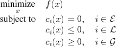

The Lagrangian function plays a fundamental role in nonlinear programming. It is used to define the optimality conditions that characterize a local minimum of the primal problem. It is also used to formulate the dual problem of the preceding primal problem. To this end, consider the following dual function:

$d(\lambda,\mu,\nu) = \inf_x\; l(x,\lambda,\mu,\nu)$

The dual problem is defined as

$l} \displaystyle\mathop\textrm{maximize}_{\lambda,\mu,\nu} & d(\lambda,\mu,\nu) \ \textrm{subject to}& \mu \le 0 \ & \nu \ge 0.$

The variables $\lambda$ , $\mu$ , and $\nu$ are called the dual variables. Note that the dual variables associated with the equality constraints ( $\lambda$ ) are free, whereas those associated with $\le$ inequality constraints ( $\mu$ ) have to be nonpositive and those associated with $\ge$ inequality constraints ( $\nu$ ) have to be nonnegative.

The relation between the primal and the dual problems provides a nice connection between the optimal solutions of the problems. Suppose is an optimal solution of the primal problem and $(\lambda^*, \mu^*, \nu^*)$ is an optimal solution of the dual problem. The difference between the objective values of the primal and dual problems, $\delta = f(x^*) - d(\lambda^*,\mu^*,\nu^*) \ge 0$ , is called the duality gap. For some restricted class of convex nonlinear programming problems, both the primal and the dual problems have an optimal solution and the optimal objective values are equal - i.e., the duality gap $\delta=0$ . In such cases, the optimal values of the dual variables correspond to the optimal Lagrange multipliers of the primal problem with the correct signs.

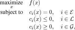
A maximization problem is treated analogously to a minimization problem. For the maximization problem

$l} \displaystyle\mathop\textrm{maximize}_{x} & f(x) \ \textrm{subject to}& c... ... & c_{i}(x) \le 0, i \in \mathcal l \ & c_{i}(x) \ge 0, i \in \mathcal g,$

the dual problem is

$l} \displaystyle\mathop\textrm{minimize}_{\lambda,\mu,\nu} & d(\lambda,\mu,\nu) \ \textrm{subject to}& \mu \ge 0 \ & \nu \le 0.$

where the dual function is defined as $\displaystyle d(\lambda,\mu,\nu)=\sup_x\; l(x,\lambda,\mu,\nu)$ and the Lagrangian function $l(x,\lambda,\mu,\nu)$ is defined the same as earlier. In this case, $\lambda$ , $\mu$ , and $-\nu$ correspond to the Lagrange multipliers in $l(x,\lambda,\mu,\nu)$ .

Minimization Problems

For inequality constraints in minimization problems, a positive optimal dual value indicates that the associated $\ge$ inequality constraint is active at the solution, and a negative optimal dual value indicates that the associated $\le$ inequality constraint is active at the solution. In PROC OPTMODEL, the optimal dual value for a range constraint (a constraint with both upper and lower bounds) is the sum of the dual values associated with the upper and lower inequalities. Since only one of the two inequalities can be active, the sign of the optimal dual value, if nonzero, identifies which one is active.

For equality constraints in minimization problems, the optimal dual values are unrestricted in sign. A positive optimal dual value for an equality constraint implies that, starting close enough to the primal solution, the same optimum could be found if the equality constraint were replaced with a $\ge$ inequality constraint. A negative optimal dual value for an equality constraint implies that the same optimum could be found if the equality constraint were replaced with a $\le$ inequality constraint.

The following is an example where simple linear programming is considered:

    proc optmodel;
       var x, y;
       min z = 6*x + 7*y;
       con 
          4*x +   y >=  5,
           -x - 3*y <= -4,
            x +   y <=  4;
       solve;
       print x y;
       expand _ACON_ ;
       print _ACON_.dual _ACON_.body;

The PRINT statements generate the output shown in Output 6.52.

The OPTMODEL Procedure

Problem Summary
Objective Sense	Minimization
Objective Function	z
Objective Type	Linear

Number of Variables	2
Bounded Above	0
Bounded Below	0
Bounded Below and Above	0
Free	2
Fixed	0

Number of Constraints	3
Linear LE (<=)	2
Linear EQ (=)	0
Linear GE (>=)	1
Linear Range	0

The OPTMODEL Procedure

Solution Summary
Solver	Dual Simplex
Objective Function	z
Solution Status	Optimal
Objective Value	13
Iterations	2

Primal Infeasibility	0
Dual Infeasibility	0
Bound Infeasibility	0

x	y
1	1

Constraint _ACON_[1]: y + 4*x >= 5                                              
 Constraint _ACON_[2]: - 3*y - x <= -4                                           
 Constraint _ACON_[3]: y + x <= 4

[1]	_ACON_.DUAL	_ACON_.BODY
1	1	5
2	-2	-4
3	0	2

Figure 6.52: Dual Values in Minimization Problem: Display

It can be seen that the first and second constraints are active, with dual values 1 and -2. Continue to submit the following statements. Notice how the objective value is changed in Output 6.53.

       _ACON_[1].lb = _ACON_[1].lb - 1;
       solve;
       _ACON_[2].ub = _ACON_[2].ub + 1;
       solve;

The OPTMODEL Procedure

Solution Summary
Solver	Dual Simplex
Objective Function	z
Solution Status	Optimal
Objective Value	12
Iterations	2

Primal Infeasibility	0
Dual Infeasibility	0
Bound Infeasibility	0

The OPTMODEL Procedure

Solution Summary
Solver	Dual Simplex
Objective Function	z
Solution Status	Optimal
Objective Value	10
Iterations	2

Primal Infeasibility	0
Dual Infeasibility	0
Bound Infeasibility	0

Figure 6.53: Dual Values in Minimization Problem: Interpretation

The change is just as the dual values imply. After the first constraint is relaxed by 1 unit, the objective value is improved by 1 unit. For the second constraint, the relaxation and improvement are 1 unit and 2 units, respectively.

CAUTION: The signs of dual values produced by PROC OPTMODEL depend, in some instances, on the way in which the corresponding constraints are entered. See the section "Constraints" for details.

Maximization Problems

For inequality constraints in maximization problems, a positive optimal dual value indicates that the associated $\le$ inequality constraint is active at the solution, and a negative optimal dual value indicates that the associated $\ge$ inequality constraint is active at the solution. The optimal dual value for a range constraint is the sum of the dual values associated with the upper and lower inequalities. The sign of the optimal dual value identifies which inequality is active.

For equality constraints in maximization problems, the optimal dual values are unrestricted in sign. A positive optimal dual value for an equality constraint implies that, starting close enough to the primal solution, the same optimum could be found if the equality constraint were replaced with a $\le$ inequality constraint. A negative optimal dual value for an equality constraint implies that the same optimum could be found if the equality constraint were replaced with a $\ge$ inequality constraint.

CAUTION: The signs of dual values produced by PROC OPTMODEL depend, in some instances, on the way in which the corresponding constraints are entered. See the section "Constraints" for details.

Top of Page