The OPTLP Procedure

Example 15.1: Oil Refinery Problem

Consider an oil refinery scenario. A step in refining crude oil into finished oil products involves a distillation process that splits crude into various streams. Suppose there are three types of crude available: Arabian light (a_l), Arabian heavy (a_h), and Brega (br). These crudes are distilled into light naphtha (na_l), intermediate naphtha (na_i), and heating oil (h_o). These in turn are blended into two types of jet fuel. Jet fuel j_1 is made up of 30% intermediate naphtha and 70% heating oil, and jet fuel j_2 is made up of 20% light naphtha and 80% heating oil. What amounts of the three crudes maximize the profit from producing jet fuel (j_1, j_2)? This problem can be formulated as the following linear program:

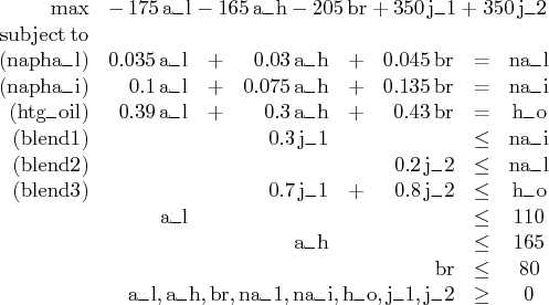
The constraints "blend1" and "blend2" ensure that j_1 and j_2 are made with the specified amounts of na_i and na_l, respectively. The constraint "blend3" is actually the reduced form of the following constraints:

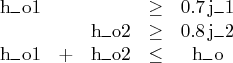
where h_o1 and h_o2 are dummy variables.

You can use the following SAS code to create the input data set ex1:

 data ex1;
 input field1 $ field2 $ field3$ field4 field5 $ field6 ;
 datalines;
 NAME        .          EX1      .     .         .
 ROWS        .          .        .     .         .
  N          profit     .        .     .         .
  E          napha_l    .        .     .         .
  E          napha_i    .        .     .         . 
  E          htg_oil    .        .     .         .
  L          blend1     .        .     .         .
  L          blend2     .        .     .         .
  L          blend3     .        .     .         .
 COLUMNS     .          .        .     .         .
 .           a_l        profit   -175  napha_l   .035
 .           a_l        napha_i  .100  htg_oil   .390
 .           a_h        profit   -165  napha_l   .030
 .           a_h        napha_i  .075  htg_oil   .300
 .           br         profit   -205  napha_l   .045
 .           br         napha_i  .135  htg_oil   .430
 .           na_l       napha_l  -1    blend2    -1
 .           na_i       napha_i  -1    blend1    -1
 .           h_o        htg_oil  -1    blend3    -1
 .           j_1        profit   350   blend1    .3
 .           j_1        blend3   .7    .         . 
 .           j_2        profit   350   blend2    .2
 .           j_2        blend3   .8    .         .
 BOUNDS      .          .        .     .         .
 UP          .          a_l      110   .         .
 UP          .          a_h      165   .         .
 UP          .          br       80    .         .
 ENDATA      .          .        .     .         .
 ;
 

You can use the following call to PROC OPTLP to solve the LP problem:

    proc optlp data=ex1 
       objsense  = max 
       solver    = primal 
       primalout = ex1pout 
       dualout   = ex1dout
       printfreq = 1;
    run;
    %put &_OROPTLP_;
 

Note that the OBJSENSE=MAX option is used to indicate that the objective function is to be maximized.

The primal and dual solutions are displayed in Output 15.1.1.

Output 15.1.1: Example 1: Primal and Dual Solution Output

The OPTLP Procedure Primal Solution Obs Objective Function ID RHS ID Variable Name Variable Type Objective Coefficient Lower Bound Upper Bound Variable Value Variable Status Reduced Cost 1 profit   a_l D -175 0 110 110.000 U 10.2083 2 profit   a_h D -165 0 165 0.000 L -22.8125 3 profit   br D -205 0 80 80.000 U 2.8125 4 profit   na_l N 0 0 1.7977E308 7.450 B 0.0000 5 profit   na_i N 0 0 1.7977E308 21.800 B 0.0000 6 profit   h_o N 0 0 1.7977E308 77.300 B 0.0000 7 profit   j_1 N 350 0 1.7977E308 72.667 B 0.0000 8 profit   j_2 N 350 0 1.7977E308 33.042 B 0.0000 The OPTLP Procedure Dual Solution Obs Objective Function ID RHS ID Constraint Name Constraint Type Constraint RHS Constraint Lower Bound Constraint Upper Bound Dual Variable Value Constraint Status Constraint Activity 1 profit   napha_l E 0 . . 0.000 L 0.00000 2 profit   napha_i E 0 . . -145.833 U 0.00000 3 profit   htg_oil E 0 . . -437.500 U 0.00000 4 profit   blend1 L 0 . . 145.833 L 0.00000 5 profit   blend2 L 0 . . 0.000 B -0.84167 6 profit   blend3 L 0 . . 437.500 L 0.00000

The progress of the solution is printed to the log as follows.

Output 15.1.2: Log: Solution Progress

NOTE: The problem EX1 has 8 variables (0 free, 0 fixed). NOTE: The problem has 6 constraints (3 LE, 3 EQ, 0 GE, 0 range). NOTE: The problem has 19 constraint coefficients. WARNING: The objective sense has been changed to maximization. NOTE: The OPTLP presolver value AUTOMATIC is applied. NOTE: The OPTLP presolver removed 3 variables and 3 constraints. NOTE: The OPTLP presolver removed 6 constraint coefficients. NOTE: The presolved problem has 5 variables, 3 constraints, and 13 constraint coefficients. NOTE: The PRIMAL SIMPLEX solver is called. Objective Entering Leaving Phase Iteration Value Variable Variable 2 1 1.5411014E-8 j_1 blend1 (S) 2 2 2.6969274E-8 j_2 blend2 (S) 2 3 5.2372044E-8 br blend3 (S) 2 4 1347.916667 blend2 (S) br NOTE: Optimal. NOTE: Objective = 1347.91667.

Note that the %put statement immediately after the OPTLP procedure prints value of the macro variable _OROPTLP_ to the log as follows.

Output 15.1.3: Log: Value of the Macro Variable _OROPTLP_

STATUS=OK SOLUTION_STATUS=OPTIMAL OBJECTIVE=1347.9166667 PRIMAL_INFEASIBILITY=2.888315E-15 DUAL_INFEASIBILITY=0 BOUND_INFEASIBILITY=0 ITERATIONS=4 PRESOLVE_TIME=0.00 SOLUTION_TIME=0.00

The value briefly summarizes the status of the OPTLP procedure upon termination.