| The NLP Procedure |
Criteria for Optimality
PROC NLP solves
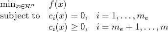
where ![]() is the objective function and the
is the objective function and the ![]() 's are
the constraint functions.
's are
the constraint functions.
A point ![]() is feasible if it satisfies all the constraints.
The feasible region
is feasible if it satisfies all the constraints.
The feasible region ![]() is the set of all the feasible points.
A feasible point
is the set of all the feasible points.
A feasible point ![]() is a global solution of the
preceding problem if no point in
is a global solution of the
preceding problem if no point in ![]() has a smaller function value than
has a smaller function value than ![]() ).
A feasible point
).
A feasible point ![]() is a local solution of the problem if there
exists some open neighborhood surrounding
is a local solution of the problem if there
exists some open neighborhood surrounding ![]() in that no point has
a smaller function value than
in that no point has
a smaller function value than ![]() ).
Nonlinear programming algorithms cannot consistently find
global minima. All the algorithms in PROC NLP find a
local minimum for this problem. If you need to check whether the obtained solution
is a global minimum, you may have to run PROC NLP with
different starting points obtained either at random or by selecting
a point on a grid that contains
).
Nonlinear programming algorithms cannot consistently find
global minima. All the algorithms in PROC NLP find a
local minimum for this problem. If you need to check whether the obtained solution
is a global minimum, you may have to run PROC NLP with
different starting points obtained either at random or by selecting
a point on a grid that contains ![]() .
.
Every local minimizer ![]() of this problem
satisfies the following local optimality conditions:
of this problem
satisfies the following local optimality conditions:
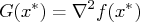
- The gradient (vector of first derivatives)
 of the objective function
  (projected toward the
feasible region if the problem is constrained) at the point
(projected toward the
feasible region if the problem is constrained) at the point  is zero.
- The Hessian (matrix of second derivatives)
 of the objective function (projected
toward the feasible region
of the objective function (projected
toward the feasible region  in the constrained case)
at the point is positive definite.
in the constrained case)
at the point is positive definite.
Most of the optimization algorithms in PROC NLP use iterative techniques
that result in a sequence of points ![]() , that
converges to a local solution
, that
converges to a local solution ![]() . At the solution, PROC NLP
performs tests to confirm that the (projected) gradient is close to
zero and that the (projected) Hessian matrix is positive definite.
. At the solution, PROC NLP
performs tests to confirm that the (projected) gradient is close to
zero and that the (projected) Hessian matrix is positive definite.
Karush-Kuhn-Tucker Conditions
An important tool in the analysis and design of algorithms in constrained optimization is the Lagrangian function, a linear combination of the objective function and the constraints:
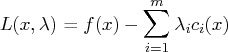
The coefficients ![]() are called Lagrange multipliers.
This tool makes it possible to state necessary and sufficient
conditions for a local minimum. The various algorithms in PROC NLP
create sequences of points, each of which is closer than the previous
one to satisfying these conditions.
are called Lagrange multipliers.
This tool makes it possible to state necessary and sufficient
conditions for a local minimum. The various algorithms in PROC NLP
create sequences of points, each of which is closer than the previous
one to satisfying these conditions.
Assuming that the functions ![]() and
and ![]() are twice continuously
differentiable, the point
are twice continuously
differentiable, the point ![]() is a local
minimum of the nonlinear programming problem, if there exists a vector
is a local
minimum of the nonlinear programming problem, if there exists a vector
![]() that meets the following
conditions.
that meets the following
conditions.
1. First-order Karush-Kuhn-Tucker conditions:
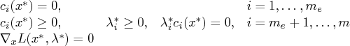
2. Second-order conditions:
Each nonzero vector ![]() that satisfies
that satisfies
Most of the algorithms to solve this problem attempt to find a
combination of vectors ![]() and
and ![]() for which the gradient
of the Lagrangian function with respect to
for which the gradient
of the Lagrangian function with respect to ![]() is zero.
is zero.
Derivatives
The first- and second-order conditions of optimality are based
on first and second derivatives of the objective function ![]() and the
constraints
and the
constraints ![]() .
.
The gradient vector contains the first
derivatives of the objective function ![]() with respect
to the parameters
with respect
to the parameters ![]() as follows:
as follows:
The ![]() symmetric Hessian matrix contains
the second derivatives of the objective function
symmetric Hessian matrix contains
the second derivatives of the objective function ![]() with
respect to the parameters
with
respect to the parameters ![]() as follows:
as follows:
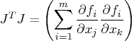
For least-squares problems, the ![]() Jacobian matrix
contains the first-order derivatives of the
Jacobian matrix
contains the first-order derivatives of the ![]() objective
functions
objective
functions ![]() with respect to the parameters
with respect to the parameters
![]() as follows:
as follows:
The ![]() Jacobian matrix contains the first-order
derivatives of the
Jacobian matrix contains the first-order
derivatives of the ![]() nonlinear constraint functions
nonlinear constraint functions ![]()
![]() , with respect to the parameters
, with respect to the parameters
![]() , as follows:
, as follows:
PROC NLP provides three ways to compute derivatives:
- It computes analytical first- and second-order derivatives
of the objective function with respect to
the
 variables
  .
. - It computes first- and second-order finite-difference approximations to the derivatives. For more information, see the section "Finite-Difference Approximations of Derivatives".
- The user supplies formulas for analytical or numerical first- and second-order derivatives of the objective function in the GRADIENT, JACOBIAN, CRPJAC, and HESSIAN statements. The JACNLC statement can be used to specify the derivatives for the nonlinear constraints.
Copyright © 2008 by SAS Institute Inc., Cary, NC, USA. All rights reserved.