The NETFLOW Procedure

Example 5.13: Machine Loading Problem

Machine loading problems arise in a variety of applications. Consider a simple instance as described in Ahuja, Magnanti, and Orlin (1993). Assume you need to schedule the production of three products, -- , on four machines, -- . Suppose that machine 1 and machine 2 are each available for 40 hours and machine 3 and machine 4 are each available for 50 hours. Also, any of the machines can produce any product. The per-unit processing time and production cost for each product on each machine are indicated in Table 5.9.

Table 5.9: Processing Times and Production Costs

---

	M1	M2	M3	M4
P1	1	2	2	3
P2	2	3	2	1
P3	3	1	2	4

---

          

---

	M1	M2	M3	M4
P1	4	3	3	1
P2	0.5	2	0.5	3
P3	2	5	1	5

---

The problem is to satisfy the demands for the three products at minimum cost.

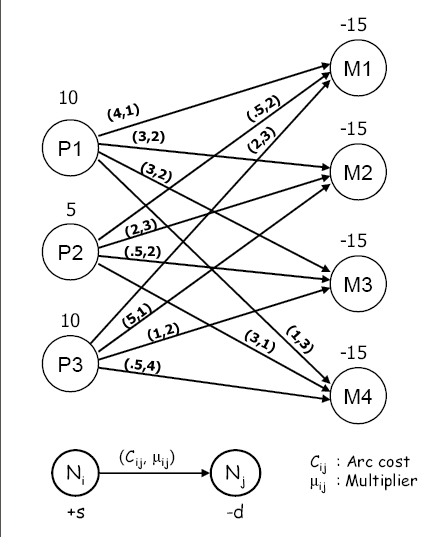
You can model this problem as a generalized network as shown in Figure 5.50. The network has three product nodes with demands indicated by positive supdem values and four machine nodes with availabilities (in hours) indicated by negative supdem values. The multiplier on an arc between a machine and a product indicates the hours of machine capacity needed to produce one unit of the product.

Figure 5.50: Machine Loading Problem

You can create the input data sets with the following SAS code:

 data mlarcs;
    input _from_ $ _to_ $ _cost_ _mult_;
 datalines;
 P1  M1   4   .
 P1  M2   3   2
 P1  M3   3   2
 P1  M4   1   3
 P2  M1  .5   2
 P2  M2   2   3
 P2  M3  .5   2
 P2  M4   3   1
 P3  M1   2   3
 P3  M2   5   .
 P3  M3   1   2
 P3  M4  .5   4
 ;
 
 data mlnodes;
    input _node_ $ _sd_;
 datalines;
 P1   10
 P2   5
 P3   10
 M1  -40
 M2  -40
 M3  -50
 M4  -50
 ;
 

You can solve the problem using the following call to PROC NETFLOW:

    title1 'The NETFLOW Procedure';
    proc netflow 
       excess   = demand
       arcdata  = mlarcs      
       nodedata = mlnodes
       conout   = mlsol;
    run;
 

The optimal solution, as displayed in Output 5.13.1, can be interpreted as follows:

• Product 1: 10 units on machine 4
• Product 2: 3 units on machine 1, and 2 units on machine 3
• Product 3: 5 units on machine 3, and 5 units on machine 4

Output 5.13.1: Optimum Solution to the Machine Loading Problem

The NETFLOW Procedure Obs _from_ _to_ _cost_ _CAPAC_ _LO_ _mult_ _SUPPLY_ _DEMAND_ _FLOW_ _FCOST_ 1 P1 M1 4.0 99999999 0 1 10 40 0.00000 0.00000 2 P2 M1 0.5 99999999 0 2 5 40 3.67856 1.83928 3 P3 M1 2.0 99999999 0 3 10 40 0.00000 0.00000 4 P1 M2 3.0 99999999 0 2 10 40 0.00000 0.00000 5 P2 M2 2.0 99999999 0 3 5 40 0.00000 0.00000 6 P3 M2 5.0 99999999 0 1 10 40 0.00000 0.00000 7 P1 M3 3.0 99999999 0 2 10 50 0.00000 0.00000 8 P2 M3 0.5 99999999 0 2 5 50 1.32144 0.66072 9 P3 M3 1.0 99999999 0 2 10 50 5.00000 5.00000 10 P1 M4 1.0 99999999 0 3 10 50 10.0000 10.0000 11 P2 M4 3.0 99999999 0 1 5 50 0.00000 0.00000 12 P3 M4 0.5 99999999 0 4 10 50 5.00000 2.50000