The NETFLOW Procedure

Example 5.10: Maximum Flow Problem

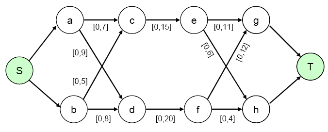
Consider the maximum flow problem depicted in Figure 5.45. The maximum flow between nodes S and T is to be determined. The minimum arc flow and arc capacities are specified as lower and upper bounds in square brackets, respectively.

Figure 5.45: Maximum Flow Problem Example

You can solve the problem using either EXCESS=ARCS or EXCESS=SLACKS. Consider using the EXCESS=ARCS option first. You can use the following SAS code to create the input data set:

 data arcs;
    input _from_ $ _to_ $ _cost_ _capac_;
 datalines;
 S a  .  .
 S b  .  .
 a c  1  7
 b c  2  9
 a d  3  5
 b d  4  8
 c e  5 15
 d f  6 20
 e g  7 11
 f g  8  6
 e h  9 12
 f h 10  4
 g T  .  .
 h T  .  .
 ;
 

You can use the following call to PROC NETFLOW to solve the problem:

    title1 'The NETFLOW Procedure';
    proc netflow 
       intpoint 
       maxflow  
       excess = arcs
       arcdata = arcs     
       source  = S    sink = T
       conout  = gout3;
    run;
 

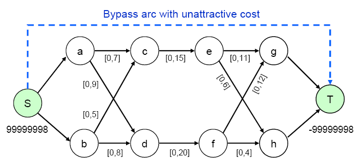
With the EXCESS=ARCS option specified, the problem gets transformed internally to the one depicted in Figure 5.46. Note that there is an additional arc from the source node to the sink node.

Figure 5.46: Maximum Flow Problem, EXCESS=ARCS Option Specified

The output SAS data set is displayed in Output 5.10.1.

Output 5.10.1: Maximum Flow Problem,EXCESS=ARCS Option Specified

The NETFLOW Procedure Obs _from_ _to_ _cost_ _capac_ _LO_ _SUPPLY_ _DEMAND_ _FLOW_ _FCOST_ 1 g T 0 99999999 0 . 99999998 16.9996 0.0000 2 h T 0 99999999 0 . 99999998 8.0004 0.0000 3 S a 0 99999999 0 99999998 . 11.9951 0.0000 4 S b 0 99999999 0 99999998 . 13.0049 0.0000 5 a c 1 7 0 . . 6.9952 6.9952 6 b c 2 9 0 . . 8.0048 16.0097 7 a d 3 5 0 . . 4.9999 14.9998 8 b d 4 8 0 . . 5.0001 20.0002 9 c e 5 15 0 . . 15.0000 75.0000 10 d f 6 20 0 . . 10.0000 60.0000 11 e g 7 11 0 . . 10.9996 76.9975 12 f g 8 6 0 . . 6.0000 48.0000 13 e h 9 12 0 . . 4.0004 36.0032 14 f h 10 4 0 . . 4.0000 40.0000

You can solve the same maximum flow problem, but this time with EXCESS=SLACKS specified. The SAS code is as follows:

    title1 'The NETFLOW Procedure';
    proc netflow 
       intpoint  
       excess  = slacks 
       arcdata = arcs
       source  = S    sink = T
       maxflow
       conout  = gout3b;
    run;
 

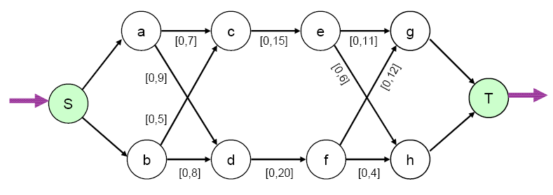
With the EXCESS=SLACKS option specified, the problem gets transformed internally to the one depicted in Figure 5.47. Note that the source node and sink node each have a single-ended "excess" arc attached to them.

Figure 5.47: Maximum Flow Problem, EXCESS=SLACKS Option Specified

The solution, as displayed in Output 5.10.2, is the same as before. Note that the _SUPPLY_ value of the source node Y has changed from 99999998 to missing S, and the _DEMAND_ value of the sink node Z has changed from -99999998 to missing D.

Output 5.10.2: Maximal Flow Problem,EXCESS=SLACKS Option Specified

The NETFLOW Procedure Obs _from_ _to_ _cost_ _capac_ _LO_ _SUPPLY_ _DEMAND_ _FLOW_ _FCOST_ 1 g T 0 99999999 0 . D 16.9993 0.0000 2 h T 0 99999999 0 . D 8.0007 0.0000 3 S a 0 99999999 0 S . 11.9867 0.0000 4 S b 0 99999999 0 S . 13.0133 0.0000 5 a c 1 7 0 . . 6.9868 6.9868 6 b c 2 9 0 . . 8.0132 16.0264 7 a d 3 5 0 . . 4.9999 14.9998 8 b d 4 8 0 . . 5.0001 20.0002 9 c e 5 15 0 . . 15.0000 75.0000 10 d f 6 20 0 . . 10.0000 60.0000 11 e g 7 11 0 . . 10.9993 76.9953 12 f g 8 6 0 . . 6.0000 48.0000 13 e h 9 12 0 . . 4.0007 36.0061 14 f h 10 4 0 . . 4.0000 40.0000