The Interior Point Nonlinear Programming Solver: Overview of Constrained Optimization :: SAS/OR(R) 9.2 User's Guide: Mathematical Programming

The Interior Point Nonlinear Programming Solver -- Experimental

Overview of Constrained Optimization

A function that plays a pivotal role in establishing conditions that characterize a local minimum of an NLP problem is the Lagrangian function $\mathcal{l}(x,y,z)$ , defined as

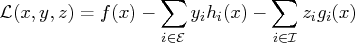
$\mathcal{l}(x,y,z) = f(x) - \sum_{i\in \mathcal{e}} y_{i} h_{i}(x) - \sum_{i\in \mathcal{i}} z_{i} g_{i}(x)$

Note that the Lagrangian function can be seen as a linear combination of the objective and constraint functions. The coefficients of the constraints, $y_{i}, i\in \mathcal{e}$ , and $z_{i}, i\in \mathcal{i}$ , are called the Lagrange multipliers or dual variables. At a feasible point $\hat{x}$ , an inequality constraint is called active if it is satisfied as an equality, i.e., $g_{i}(\hat{x}) = 0$ . The set of active constraints at a feasible point $\hat{x}$ is then defined as the union of the index set of the equality constraints, $\mathcal{e}$ , and the indices of those inequality constraints that are active at $\hat{x}$ , i.e.,

$\mathcal{a}(\hat{x}) = \mathcal{e} \cup \{ i\in \mathcal{i}: g_{i}(\hat{x}) = 0 \}$

An important condition that is assumed to hold in the majority of optimization algorithms is the so-called linear independence constraint qualification (LICQ). The LICQ states that at any feasible point $\hat{x}$ , the gradients of all the active constraints are linearly independent. The main purpose of the LICQ is to ensure that the set of constraints is well-defined, in a way that there are no redundant constraints, or in a way that there are no constraints defined such that their gradients are always equal to zero.

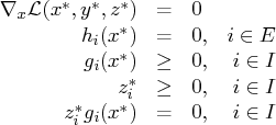
The First-Order Necessary Optimality Conditions

If $x^{*}$ is a local minimum of the NLP problem and the LICQ holds at $x^{*}$ , then there are vectors of Lagrange multipliers $y^{*}$ and $z^{*}$ , with components $y_{i}^{*}, i \in \mathcal{e}$ , and $z_{i}^{*}, i \in \mathcal{i}$ , respectively, such that the following conditions are satisfied:

$\nabla_{x} \mathcal{l}(x^{*}, y^{*}, z^{*}) &=&0 & \ h_{i}(x^{*}) &=&0, & i \in... ... \in i \ z_{i}^{*} &\ge&0, & i \in i \ z_{i}^{*} g_{i}(x^{*}) &=&0, & i \in i$

where $\nabla_{x} \mathcal{l}(x^{*}, y^{*}, z^{*})$ is the gradient of the Lagrangian function with respect to

, defined as

$\nabla_{x} \mathcal{l}(x^{*}, y^{*}, z^{*}) = \nabla f(x) - \sum_{i\in \mathcal{e}} y_{i} \nabla h_{i}(x) - \sum_{i\in \mathcal{i}} z_{i} \nabla g_{i}(x)$

The preceding conditions are often called the Karush-Kuhn-Tucker (KKT) conditions , named after their inventors. The last group of equations ( $z_{i} g_{i}(x) = 0, i \in i$ ) is called the complementarity condition. Its main aim is to try to force the Lagrange multipliers, $z_{i}^{*}$ , of the inactive inequalities (i.e., those inequalities with $g_{i}(x^{*}) \gt 0$ ) to zero.

The KKT conditions describe the way the first derivatives of the objective and constraints are related at a local minimum $x^{*}$ . However, they are not enough to fully characterize a local minimum. The second-order optimality conditions attempt to fulfill this aim, by examining the curvature of the Hessian matrix of the Lagrangian function at a point that satisfies the KKT conditions.

The Second-Order Necessary Optimality Condition

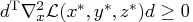
Let $x^{*}$ be a local minimum of the NLP problem, and let $y^{*}, z^{*}$ be the corresponding Lagrange multipliers that satisfy the first-order optimality conditions. Then $d^{\rm t} \nabla_{x}^2 \mathcal{l}(x^{*},y^{*},z^{*}) d \ge 0$ for all nonzero vectors

that satisfy the following conditions:

$\nabla h_{i}^{\rm t} (x^{*})d = 0$ , $\forall i\in \mathcal{e}$
$\nabla g_{i}^{\rm t} (x^{*})d = 0$ , $\forall i\in \mathcal{a}(x^{*})$ , such that $z_{i}^{*} \gt 0$
$\nabla g_{i}^{\rm t} (x^{*})d \ge 0$ , $\forall i\in \mathcal{a}(x^{*})$ , such that $z_{i}^{*} = 0$

The second-order necessary optimality condition states that, at a local minimum, the curvature of the Lagrangian function along the directions that satisfy the preceding conditions must be nonnegative.

Top of Page