| The INTPOINT Procedure |
Getting Started: NPSC Problems
To solve NPSC problems using PROC INTPOINT, you save a representation of the network and the side constraints in three SAS data sets. These data sets are then passed to PROC INTPOINT for solution. There are various forms that a problem's data can take. You can use any one or a combination of several of these forms.
The NODEDATA= data set contains the names of
the supply and demand
nodes and the supply or demand associated with each.
These are the elements in the column vector
![]() in the NPSC problem (see the section "Mathematical Description of NPSC").
in the NPSC problem (see the section "Mathematical Description of NPSC").
The ARCDATA= data set contains information about the variables of the problem. Usually these are arcs, but there can be data related to nonarc variables in the ARCDATA= data set as well.
An arc is identified by the names of its tail node (where it
originates) and head node (where it is directed).
Each observation can be used to identify an arc in the network and,
optionally, the cost per flow unit across the arc, the arc's
capacity, lower flow bound, and name.
These data are associated with the matrix ![]() and
the vectors
and
the vectors ![]() ,
, ![]() , and
, and ![]() in the NPSC
problem (see the section "Mathematical Description of NPSC").
in the NPSC
problem (see the section "Mathematical Description of NPSC").
Note: Although
![]() is a node-arc incidence matrix, it is specified
in the ARCDATA= data set by arc
definitions.
Do not explicitly specify these flow conservation constraints as
constraints of the problem.
is a node-arc incidence matrix, it is specified
in the ARCDATA= data set by arc
definitions.
Do not explicitly specify these flow conservation constraints as
constraints of the problem.
In addition,
the ARCDATA= data set can be used to specify information about
nonarc variables, including objective function coefficients,
lower and upper value bounds, and names.
These data are the elements of the vectors
![]() ,
, ![]() , and
, and ![]() in the NPSC problem (see the section "Mathematical Description of NPSC").
Data for an arc or nonarc variable can be given in more than
one observation.
in the NPSC problem (see the section "Mathematical Description of NPSC").
Data for an arc or nonarc variable can be given in more than
one observation.
Supply and demand data also can be specified in the ARCDATA= data set. In such a case, the NODEDATA= data set may not be needed.
The CONDATA= data set describes the side constraints and
their right-hand sides. These data are elements of the matrices ![]() and
and
![]() and
the vector
and
the vector ![]() .
Constraint types are also specified in the CONDATA= data set.
You can include in this data set upper bound values or capacities,
lower flow or value bounds, and costs or objective function
coefficients. It is possible to give all information about
some or all nonarc variables in the CONDATA= data set.
.
Constraint types are also specified in the CONDATA= data set.
You can include in this data set upper bound values or capacities,
lower flow or value bounds, and costs or objective function
coefficients. It is possible to give all information about
some or all nonarc variables in the CONDATA= data set.
An arc is identified in this data set by its name. If you specify an arc's name in the ARCDATA= data set, then this name is used to associate data in the CONDATA= data set with that arc. Each arc also has a default name that is the name of the tail and head node of the arc concatenated together and separated by an underscore character; tail_head, for example.
If you use the dense side constraint input format (described in the section "CONDATA= Data Set"), and want to use the default arc names, these arc names are names of SAS variables in the VAR list of the CONDATA= data set.
If you use the sparse side constraint input format (see the section "CONDATA= Data Set") and want to use the default arc names, these arc names are values of the COLUMN list variable of the CONDATA= data set.
PROC INTPOINT reads the data from the NODEDATA= data set, the ARCDATA= data set, and the CONDATA= data set. Error checking is performed, and the model is converted into an equivalent LP. This LP is preprocessed. Preprocessing is optional but highly recommended. Preprocessing analyzes the model and tries to determine before optimization whether variables can be "fixed" to their optimal values. Knowing that, the model can be modified and these variables dropped out. It can be determined that some constraints are redundant. Sometimes, preprocessing succeeds in reducing the size of the problem, thereby making the subsequent optimization easier and faster.
The optimal solution to the equivalent LP is then found. This LP is converted back to the original NPSC problem, and the optimum for this is derived from the optimum of the equivalent LP. If the problem was preprocessed, the model is now post-processed, where fixed variables are reintroduced. The solution can be saved in the CONOUT= data set.
Introductory NPSC Example
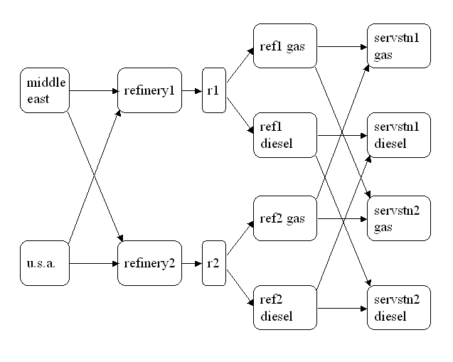
Consider the following transshipment problem for an oil company. Crude oil is shipped to refineries where it is processed into gasoline and diesel fuel. The gasoline and diesel fuel are then distributed to service stations. At each stage, there are shipping, processing, and distribution costs. Also, there are lower flow bounds and capacities.In addition, there are two sets of side constraints. The first set is that two times the crude from the Middle East cannot exceed the throughput of a refinery plus 15 units. (The phrase "plus 15 units" that finishes the last sentence is used to enable some side constraints in this example to have a nonzero rhs.) The second set of constraints are necessary to model the situation that one unit of crude mix processed at a refinery yields three-fourths of a unit of gasoline and one-fourth of a unit of diesel fuel.
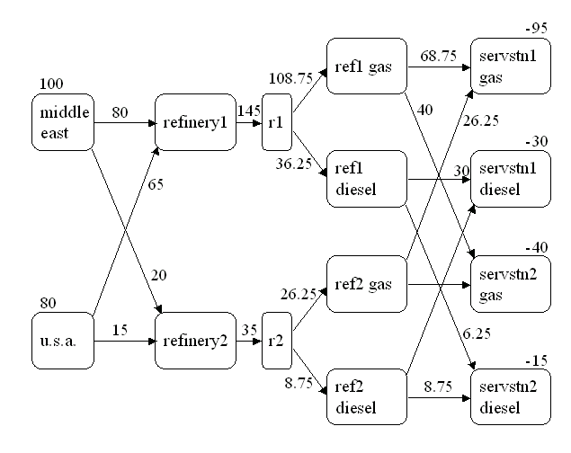
Because there are two products that are not independent in the way in which they flow through the network, an NPSC is an appropriate model for this example (see Figure 2.6). The side constraints are used to model the limitations on the amount of Middle Eastern crude that can be processed by each refinery and the conversion proportions of crude to gasoline and diesel fuel.
|
Figure 2.6: Oil Industry Example
To solve this problem with PROC INTPOINT, save a representation
of the model in three SAS data sets.
In the NODEDATA= data set, you name the supply
and demand nodes and give the associated supplies and demands.
To distinguish
demand nodes from supply nodes, specify demands
as negative quantities. For the oil example, the NODEDATA= data set
can be saved as follows:
    title  'Oil Industry Example';
    title3 'Setting Up Nodedata = Noded For PROC INTPOINT';
    data noded;
       input   _node_&$15. _sd_;
       datalines;
    middle east       100
    u.s.a.             80
    servstn1 gas      -95
    servstn1 diesel   -30
    servstn2 gas      -40
    servstn2 diesel   -15
    ;
The ARCDATA= data set contains the rest of the information about the network. Each observation in the data set identifies an arc in the network and gives the cost per flow unit across the arc, the capacities of the arc, the lower bound on flow across the arc, and the name of the arc.
    title3 'Setting Up Arcdata = Arcd1 For PROC INTPOINT';
    data arcd1;
       input _from_&$11. _to_&$15. _cost_ _capac_ _lo_ _name_ $;
       datalines;
    middle east    refinery 1        63     95   20    m_e_ref1
    middle east    refinery 2        81     80   10    m_e_ref2
    u.s.a.         refinery 1        55      .    .    .
    u.s.a.         refinery 2        49      .    .    .
    refinery 1     r1               200    175   50    thruput1
    refinery 2     r2               220    100   35    thruput2
    r1             ref1 gas           .    140    .    r1_gas
    r1             ref1 diesel        .     75    .    .
    r2             ref2 gas           .    100    .    r2_gas
    r2             ref2 diesel        .     75    .    .
    ref1 gas       servstn1 gas      15     70    .    .
    ref1 gas       servstn2 gas      22     60    .    .
    ref1 diesel    servstn1 diesel   18      .    .    .
    ref1 diesel    servstn2 diesel   17      .    .    .
    ref2 gas       servstn1 gas      17     35    5    .
    ref2 gas       servstn2 gas      31      .    .    .
    ref2 diesel    servstn1 diesel   36      .    .    .
    ref2 diesel    servstn2 diesel   23      .    .    .
    ;
Finally, the CONDATA= data set contains the side constraints for the model:
    title3 'Setting Up Condata = Cond1 For PROC INTPOINT';
    data cond1;
       input m_e_ref1 m_e_ref2 thruput1 r1_gas thruput2 r2_gas
             _type_ $ _rhs_;
       datalines;
    -2  .  1 .  . . >= -15
     . -2  . .  1 . GE -15
     .  . -3 4  . . EQ   0
     .  .  . . -3 4  =   0
    ;
Note that the SAS variable names in the CONDATA= data set are the names of arcs given in the ARCDATA= data set. These are the arcs that have nonzero constraint coefficients in side constraints. For example, the proportionality constraint that specifies that one unit of crude at each refinery yields three-fourths of a unit of gasoline and one-fourth of a unit of diesel fuel is given for refinery 1 in the third observation and for refinery 2 in the last observation. The third observation requires that each unit of flow on the arc thruput1 equals three-fourths of a unit of flow on the arc r1_gas. Because all crude processed at refinery 1 flows through thruput1 and all gasoline produced at refinery 1 flows through r1_gas, the constraint models the situation. It proceeds similarly for refinery 2 in the last observation.
To find the minimum cost flow through the network that satisfies the supplies, demands, and side constraints, invoke PROC INTPOINT as follows:
    proc intpoint
       bytes=1000000
       nodedata=noded        /* the supply and demand data */
       arcdata=arcd1         /* the arc descriptions       */
       condata=cond1         /* the side constraints       */
       conout=solution;      /* the solution data set      */
       run;
The following messages, which appear on the SAS log, summarize the model as read by PROC INTPOINT and note the progress toward a solution.
    NOTE: Number of nodes= 14 .
    NOTE: Number of supply nodes= 2 .
    NOTE: Number of demand nodes= 4 .
    NOTE: Total supply= 180 , total demand= 180 .
    NOTE: Number of arcs= 18 .
    NOTE: Number of <= side constraints= 0 .
    NOTE: Number of == side constraints= 2 .
    NOTE: Number of >= side constraints= 2 .
    NOTE: Number of side constraint coefficients= 8 .
    NOTE: The following messages relate to the equivalent
          Linear Programming problem solved by the Interior
          Point algorithm.
    NOTE: Number of <= constraints= 0 .
    NOTE: Number of == constraints= 16 .
    NOTE: Number of >= constraints= 2 .
    NOTE: Number of constraint coefficients= 44 .
    NOTE: Number of variables= 18 .
    NOTE: After preprocessing, number of <= constraints= 0.
    NOTE: After preprocessing, number of == constraints= 5.
    NOTE: After preprocessing, number of >= constraints= 2.
    NOTE: The preprocessor eliminated 11 constraints from the
          problem.
    NOTE: The preprocessor eliminated 25 constraint
          coefficients from the problem.
    NOTE: After preprocessing, number of variables= 8.
    NOTE: The preprocessor eliminated 10 variables from the
          problem.
    NOTE: 2 columns, 0 rows and 2 coefficients were added to
          the problem to handle unrestricted variables,
          variables that are split, and constraint slack or
          surplus variables.
    NOTE: There are 13 nonzero elements in A * A transpose.
    NOTE: Of the 7 rows and columns, 2 are sparse.
    NOTE: There are 6 nonzero superdiagonal elements in the
          sparse rows of the factored A * A transpose. This
          includes fill-in.
    NOTE: There are 2 operations of the form
          u[i,j]=u[i,j]-u[q,j]*u[q,i]/u[q,q] to factorize the
          sparse rows of A * A transpose.
    NOTE: Bound feasibility attained by iteration 1.
    NOTE: Dual feasibility attained by iteration 1.
    NOTE: Constraint feasibility attained by iteration 2.
    NOTE: The Primal-Dual Predictor-Corrector Interior Point
          algorithm performed 7 iterations.
    NOTE: Objective = 50875.01279.
    NOTE: The data set WORK.SOLUTION has 18 observations and
          10 variables.
    NOTE: There were 18 observations read from the data set
          WORK.ARCD1.
    NOTE: There were 6 observations read from the data set
          WORK.NODED.
    NOTE: There were 4 observations read from the data set
          WORK.COND1.
The first set of messages shows the size of the problem. The next set of messages provides statistics on the size of the equivalent LP problem. The number of variables may not equal the number of arcs if the problem has nonarc variables. This example has none. To convert a network to the equivalent LP problem, a flow conservation constraint must be created for each node (including an excess or bypass node, if required). This explains why the number of equality constraints and the number of constraint coefficients differ from the number of equality side constraints and the number of coefficients in all side constraints.
If the preprocessor was successful in decreasing the problem size, some messages will report how well it did. In this example, the model size was cut approximately in half!
The next set of messages describes aspects of the interior point algorithm.
Of particular interest are those concerned with
the Cholesky factorization of
![]() where
where ![]() is the coefficient matrix of the final LP.
It is crucial to preorder the rows and columns of this matrix to prevent
fill-in and reduce the number of row operations to undertake
the factorization.
See the section "Interior Point Algorithmic Details" for a more extensive explanation.
is the coefficient matrix of the final LP.
It is crucial to preorder the rows and columns of this matrix to prevent
fill-in and reduce the number of row operations to undertake
the factorization.
See the section "Interior Point Algorithmic Details" for a more extensive explanation.
Unlike PROC LP, which displays the solution and other information as output, PROC INTPOINT saves the optimum in the output SAS data set that you specify. For this example, the solution is saved in the SOLUTION data set. It can be displayed with the PRINT procedure as
    title3 'Optimum';
    proc print data=solution;
       var _from_ _to_ _cost_ _capac_ _lo_ _name_
           _supply_ _demand_ _flow_ _fcost_;
       sum _fcost_;
       run;
Figure 2.7: CONOUT=SOLUTION
Notice that, in CONOUT=SOLUTION (Figure 2.7), the optimal flow through each arc in the network is given in the variable named _FLOW_, and the cost of flow through each arc is given in the variable _FCOST_.
|
Copyright © 2008 by SAS Institute Inc., Cary, NC, USA. All rights reserved.