The NETFLOW Procedure
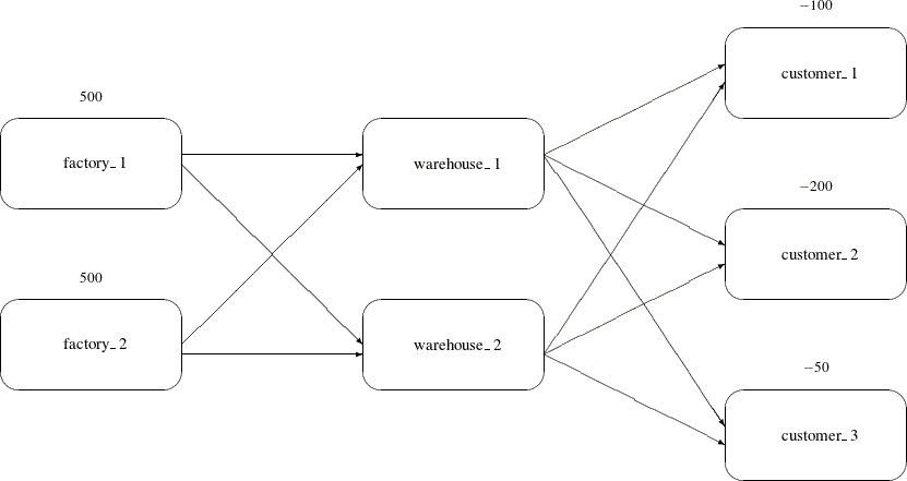
Network flow problems can be described by specifying the nodes in the network and their supplies and demands, specifying the arcs in the network and their costs, capacities, and lower flow bounds. Consider the simple transshipment problem in Figure 4.3 as an illustration.
Figure 4.3: Transshipment Problem

Suppose the candy manufacturing company has two factories, two warehouses, and three customers for chocolate. The two factories each have a production capacity of 500 pounds per day. The three customers have demands of 100, 200, and 50 pounds per day, respectively.
The following data set describes the supplies (positive values for the supdem variable) and the demands (negative values for the supdem variable) for each of the customers and factories:
data nodes;
format node $10. ;
input node $ supdem;
datalines;
customer_1   -100
customer_2   -200
customer_3    -50
factory_1     500
factory_2     500
;
Suppose that two warehouses are used to store the chocolate before shipment to the customers, and that there are different costs for shipping between each factory, warehouse, and customer. What is the minimum cost routing for supplying the customers?
Arcs are described in another data set. Each observation defines a new arc in the network and gives data about the arc. For example, there is an arc between the node factory_1 and the node warehouse_1. Each unit of flow on that arc costs 10. Although this example does not include it, lower and upper bounds on the flow across that arc can also be listed here.
data network;
   format from $12. to $12.;
   input from $ to $ cost ;
   datalines;
factory_1     warehouse_1  10
factory_2     warehouse_1   5
factory_1     warehouse_2   7
factory_2     warehouse_2   9
warehouse_1   customer_1    3
warehouse_1   customer_2    4
warehouse_1   customer_3    4
warehouse_2   customer_1    5
warehouse_2   customer_2    5
warehouse_2   customer_3    6
;
You can use PROC NETFLOW to find the minimum cost routing. This procedure takes the model as defined in the network and nodes data sets and finds the minimum cost flow.
proc netflow arcout=arc_sav
             arcdata=network nodedata=nodes;
   node node;      /* node data set information */
   supdem supdem;
   tail from;      /* arc data set information */
   head to;
   cost cost;
   run;
proc print;
   var from to cost _capac_ _lo_ _supply_ _demand_
       _flow_ _fcost_ _rcost_;
   sum _fcost_;
   run;
PROC NETFLOW produces the following messages in the SAS log:
| NOTE: Number of nodes= 7 . |
| NOTE: Number of supply nodes= 2 . |
| NOTE: Number of demand nodes= 3 . |
| NOTE: Total supply= 1000 , total demand= 350 . |
| NOTE: Number of arcs= 10 . |
| NOTE: Number of iterations performed (neglecting any constraints)= 9 . |
| NOTE: Of these, 2 were degenerate. |
| NOTE: Optimum (neglecting any constraints) found. |
| NOTE: Minimal total cost= 3050 . |
| NOTE: The data set WORK.ARC_SAV has 10 observations and 13 variables. |
The solution (Figure 4.4) saved in the arc_sav data set shows the optimal amount of chocolate to send across each arc (the amount to ship from each factory to each warehouse
and from each warehouse to each customer) in the network per day.
Figure 4.4: ARCOUT Data Set
| Obs | from | to | cost | _CAPAC_ | _LO_ | _SUPPLY_ | _DEMAND_ | _FLOW_ | _FCOST_ | _RCOST_ |
|---|---|---|---|---|---|---|---|---|---|---|
| 1 | warehouse_1 | customer_1 | 3 | 99999999 | 0 | . | 100 | 100 | 300 | . |
| 2 | warehouse_2 | customer_1 | 5 | 99999999 | 0 | . | 100 | 0 | 0 | 4 |
| 3 | warehouse_1 | customer_2 | 4 | 99999999 | 0 | . | 200 | 200 | 800 | . |
| 4 | warehouse_2 | customer_2 | 5 | 99999999 | 0 | . | 200 | 0 | 0 | 3 |
| 5 | warehouse_1 | customer_3 | 4 | 99999999 | 0 | . | 50 | 50 | 200 | . |
| 6 | warehouse_2 | customer_3 | 6 | 99999999 | 0 | . | 50 | 0 | 0 | 4 |
| 7 | factory_1 | warehouse_1 | 10 | 99999999 | 0 | 500 | . | 0 | 0 | 5 |
| 8 | factory_2 | warehouse_1 | 5 | 99999999 | 0 | 500 | . | 350 | 1750 | . |
| 9 | factory_1 | warehouse_2 | 7 | 99999999 | 0 | 500 | . | 0 | 0 | . |
| 10 | factory_2 | warehouse_2 | 9 | 99999999 | 0 | 500 | . | 0 | 0 | 2 |
| 3050 |
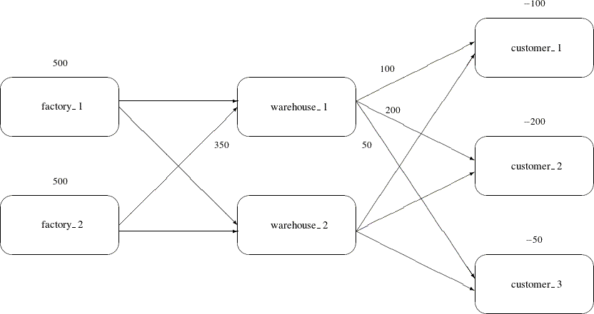
Notice which arcs have positive flow (_FLOW_ is greater than 0). These arcs indicate the amount of chocolate that should be sent from factory_2 to warehouse_1 and from
there to the three customers. The solution indicates no production at factory_1 and no use of warehouse_2.
Figure 4.5: Optimal Solution for the Transshipment Problem
