PROC INTPOINT: Network Models

Network Models

The following are descriptions of some typical NPSC models.

Production, Inventory, and Distribution (Supply Chain) Problems

One common class of network models is the production-inventory-distribution or supply-chain problem. The diagram in Figure 4.1 illustrates this problem. The subscripts on the Production, Inventory, and Sales nodes indicate the time period. By replicating sections of the model, the notion of time can be included.

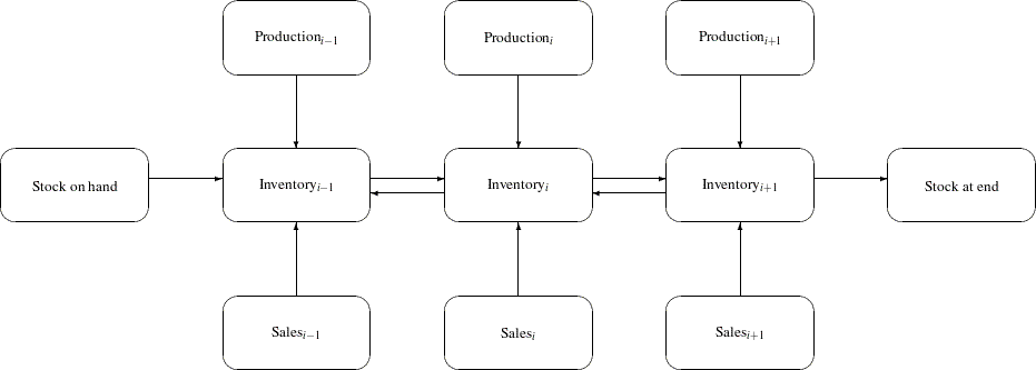
Figure 4.1 Production-Inventory-Distribution Problem

In this type of model, the nodes can represent a wide variety of facilities. Several examples are suppliers, spot markets, importers, farmers, manufacturers, factories, parts of a plant, production lines, waste disposal facilities, workstations, warehouses, coolstores, depots, wholesalers, export markets, ports, rail junctions, airports, road intersections, cities, regions, shops, customers, and consumers. The diversity of this selection demonstrates how rich the potential applications of this model are.

Depending upon the interpretation of the nodes, the objectives of the modeling exercise can vary widely. Some common types of objectives are

to reduce collection or purchase costs of raw materials
to reduce inventory holding or backorder costs. Warehouses and other storage facilities sometimes have capacities, and there can be limits on the amount of goods that can be placed on backorder.
to decide where facilities should be located and what the capacity of these should be. Network models have been used to help decide where factories, hospitals, ambulance and fire stations, oil and water wells, and schools should be sited.
to determine the assignment of resources (machines, production capability, workforce) to tasks, schedules, classes, or files
to determine the optimal distribution of goods or services. This usually means minimizing transportation costs and reducing transit time or distances covered.
to find the shortest path from one location to another
to ensure that demands (for example, production requirements, market demands, contractual obligations) are met
to maximize profits from the sale of products or the charge for services
to maximize production by identifying bottlenecks

Some specific applications are

car distribution models. These help determine which models and numbers of cars should be manufactured in which factories and where to distribute cars from these factories to zones in the United States in order to meet customer demand at least cost.
models in the timber industry. These help determine when to plant and mill forests, schedule production of pulp, paper, and wood products, and distribute products for sale or export.
military applications. The nodes can be theaters, bases, ammunition dumps, logistical suppliers, or radar installations. Some models are used to find the best ways to mobilize personnel and supplies and to evacuate the wounded in the least amount of time.
communications applications. The nodes can be telephone exchanges, transmission lines, satellite links, and consumers. In a model of an electrical grid, the nodes can be transformers, powerstations, watersheds, reservoirs, dams, and consumers. The effect of high loads or outages might be of concern.

Proportionality Constraints

In many models, you have the characteristic that a flow through an arc must be proportional to the flow through another arc. Side constraints are often necessary to model that situation. Such constraints are called proportionality constraints and are useful in models where production is subject to refining or modification into different materials. The amount of each output, or any waste, evaporation, or reduction can be specified as a proportion of input.

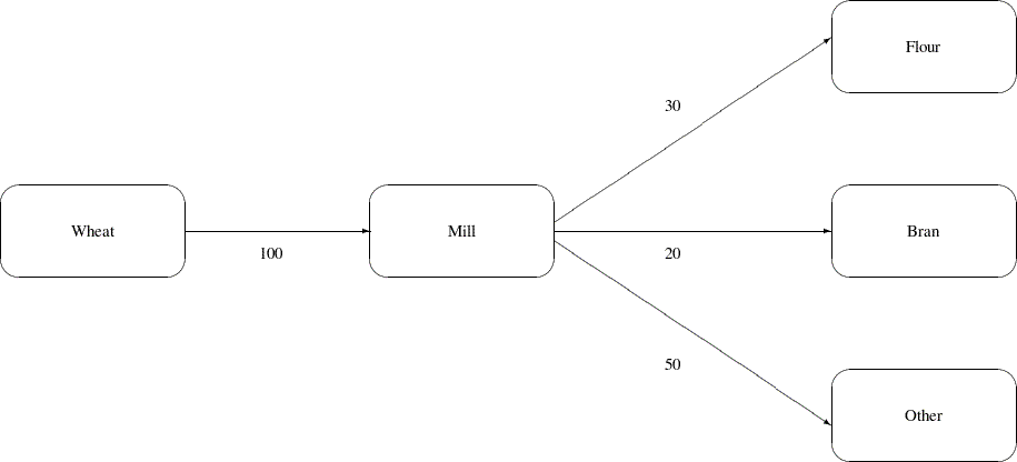
Typically, the arcs near the supply nodes carry raw materials and the arcs near the demand nodes carry refined products. For example, in a model of the milling industry, the flow through some arcs may represent quantities of wheat. After the wheat is processed, the flow through other arcs might be flour. For others it might be bran. The side constraints model the relationship between the amount of flour or bran produced as a proportion of the amount of wheat milled. Some of the wheat can end up as neither flour, bran, nor any useful product, so this waste is drained away via arcs to a waste node.

Figure 4.2 Proportionality Constraints

In order for arcs to be specified in side constraints, they must be named. By default, PROC INTPOINT names arcs using the names of the nodes at the head and tail of the arc. An arc is named with its tail node name followed by an underscore and its head node name. For example, an arc from node from to node to is called from_to.

Consider the network fragment in Figure 4.2. The arc Wheat_Mill conveys the wheat milled. The cost of flow on this arc is the milling cost. The capacity of this arc is the capacity of the mill. The lower flow bound on this arc is the minimum quantity that must be milled for the mill to operate economically. The constraints

$\text{[math]}$ Wheat_Mill $\text{[math]}$ Mill_Flour $\text{[math]}$
$\text{[math]}$ Wheat_Mill $\text{[math]}$ Mill_Bran $\text{[math]}$

force every unit of wheat that is milled to produce 0.3 units of flour and 0.2 units of bran. Note that it is not necessary to specify the constraint

$\text{[math]}$ Wheat_Mill $\text{[math]}$ Mill_Other $\text{[math]}$

since flow conservation implies that any flow that does not traverse through Mill_Flour or Mill_Bran must be conveyed through Mill_Other. And, computationally, it is better if this constraint is not specified, since there is one less side constraint and fewer problems with numerical precision. Notice that the sum of the proportions must equal 1.0 exactly; otherwise, flow conservation is violated.

Blending Constraints

Blending or quality constraints can also influence the recipes or proportions of ingredients that are mixed. For example, different raw materials can have different properties. In an application of the oil industry, the amount of products that are obtained could be different for each type of crude oil. Furthermore, fuel might have a minimum octane requirement or limited sulphur or lead content, so that a blending of crudes is needed to produce the product.

The network fragment in Figure 4.3 shows an example of this.

Figure 4.3 Blending Constraints

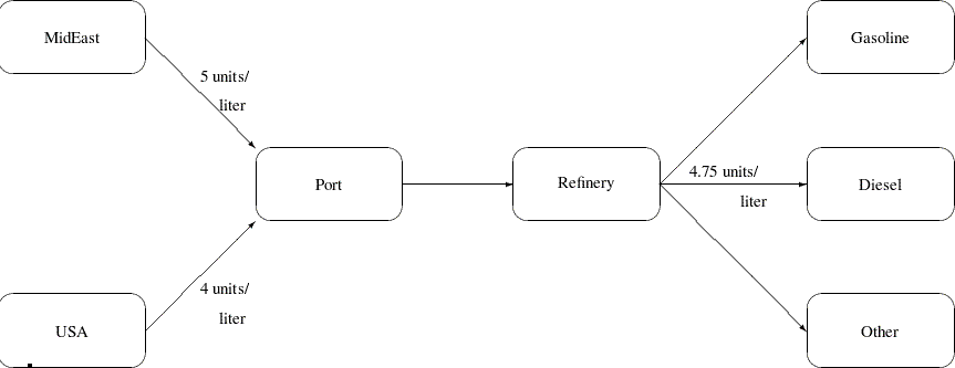
The arcs MidEast_Port and USA_Port convey crude oil from the two sources. The arc Port_Refinery represents refining while the arcs Refinery_Gasoline and Refinery_Diesel carry the gas and diesel produced. The proportionality constraints

$\text{[math]}$ Port_Refinery $\text{[math]}$ Refinery_Gasoline $\text{[math]}$
$\text{[math]}$ Port_Refinery $\text{[math]}$ Refinery_Diesel $\text{[math]}$

capture the restrictions for producing gasoline and diesel from crude. Suppose that only crude from the Middle East is used, then the resulting diesel would contain 5 units of sulphur per liter. If only crude from the U.S.A. is used, the resulting diesel would contain 4 units of sulphur per liter. Diesel can have at most 4.75 units of sulphur per liter. Some crude from the U.S.A. must be used if Middle East crude is used in order to meet the 4.75 sulphur per liter limit. The side constraint to model this requirement is

$\text{[math]}$ MidEast_Port $\text{[math]}$ USA_Port $\text{[math]}$ Port_Refinery $\text{[math]}$ $\text{[math]}$

Since Port_Refinery $\text{[math]}$ MidEast_Port $\text{[math]}$ USA_Port, flow conservation allows this constraint to be simplified to

$\text{[math]}$ MidEast_Port $\text{[math]}$ USA_Port $\text{[math]}$ $\text{[math]}$

If, for example, 120 units of crude from the Middle East is used, then at least 40 units of crude from the U.S.A. must be used. The preceding constraint is simplified because you assume that the sulphur concentration of diesel is proportional to the sulphur concentration of the crude mix. If this is not the case, the relation

$\text{[math]}$ Port_Refinery $\text{[math]}$ Refinery_Diesel

is used to obtain

$\text{[math]}$ MidEast_Port $\text{[math]}$ USA_Port $\text{[math]}$ Refinery_Diesel $\text{[math]}$ $\text{[math]}$ $\text{[math]}$

which equals

$\text{[math]}$ MidEast_Port $\text{[math]}$ USA_Port $\text{[math]}$ Refinery_Diesel $\text{[math]}$ $\text{[math]}$

An example similar to this oil industry problem is solved in the section Introductory NPSC Example.

Multicommodity Problems

Side constraints are also used in models in which there are capacities on transportation or some other shared resource, or there are limits on overall production or demand in multicommodity, multidivisional, or multiperiod problems. Each commodity, division, or period can have a separate network coupled to one main system by the side constraints. Side constraints are used to combine the outputs of subdivisions of a problem (either commodities, outputs in distinct time periods, or different process streams) to meet overall demands or to limit overall production or expenditures. This method is more desirable than doing separate local optimizations for individual commodity, process, or time networks and then trying to establish relationships between each when determining an overall policy if the global constraint is not satisfied. Of course, to make models more realistic, side constraints may be necessary in the local problems.

Figure 4.4 Multicommodity Problem

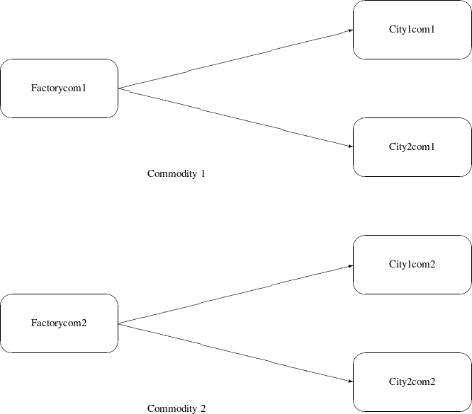
Figure 4.4 shows two network fragments. They represent identical production and distribution sites of two different commodities. Suffix com1 represents commodity 1 and suffix com2 represents commodity 2. The nodes Factorycom1 and Factorycom2 model the same factory, and nodes City1com1 and City1com2 model the same location, city 1. Similarly, City2com1 and City2com2 are the same location, city 2. Suppose that commodity 1 occupies 2 cubic meters, commodity 2 occupies 3 cubic meters, the truck dispatched to city 1 has a capacity of 200 cubic meters, and the truck dispatched to city 2 has a capacity of 250 cubic meters. How much of each commodity can be loaded onto each truck? The side constraints for this case are

$\text{[math]}$ Factorycom1_City1com1 $\text{[math]}$ Factorycom2_City1com2 $\text{[math]}$ $\text{[math]}$
$\text{[math]}$ Factorycom1_City2com1 $\text{[math]}$ Factorycom2_City2com2 $\text{[math]}$ $\text{[math]}$

Large Modeling Strategy

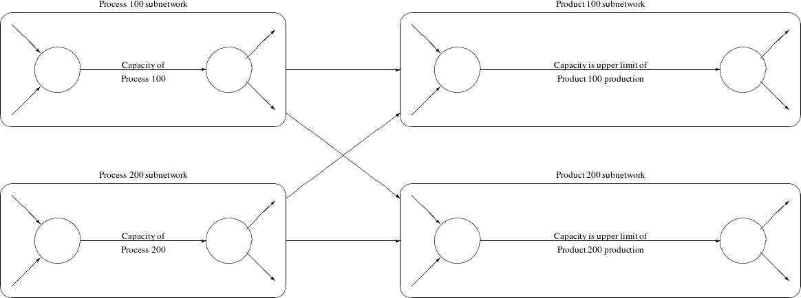
In many cases, the flow through an arc might actually represent the flow or movement of a commodity from place to place or from time period to time period. However, sometimes an arc is included in the network as a method of capturing some aspect of the problem that you would not normally think of as part of a network model. There is no commodity movement associated with that arc. For example, in a multiprocess, multiproduct model (Figure 4.5), there might be subnetworks for each process and each product. The subnetworks can be joined together by a set of arcs that have flows that represent the amount of product $\text{[math]}$ produced by process $\text{[math]}$ . To model an upper-limit constraint on the total amount of product $\text{[math]}$ that can be produced, direct all arcs carrying product $\text{[math]}$ to a single node and from there through a single arc. The capacity of this arc is the upper limit of product $\text{[math]}$ production. It is preferable to model this structure in the network rather than to include it in the side constraints because the efficiency of the optimizer may be less affected by a reasonable increase in the size of the network rather than increasing the number or complicating side constraints.

Figure 4.5 Multiprocess, Multiproduct Example

When starting a project, it is often a good strategy to use a small network formulation and then use that model as a framework upon which to add detail. For example, in the multiprocess, multiproduct model, you might start with the network depicted in Figure 4.5. Then, for example, the process subnetwork can be enhanced to include the distribution of products. Other phases of the operation could be included by adding more subnetworks. Initially, these subnetworks can be single nodes, but in subsequent studies they can be expanded to include greater detail.

Advantages of Network Models over LP Models

Many linear programming problems have large embedded network structures. Such problems often result when modeling manufacturing processes, transportation or distribution networks, or resource allocation, or when deciding where to locate facilities. Often, some commodity is to be moved from place to place, so the more natural formulation in many applications is that of a constrained network rather than a linear program.

Using a network diagram to visualize a problem makes it possible to capture the important relationships in an easily understood picture form. The network diagram aids the communication between model builder and model user, making it easier to comprehend how the model is structured, how it can be changed, and how results can be interpreted.

If a network structure is embedded in a linear program, the problem is an NPSC (see the section Mathematical Description of NPSC). When the network part of the problem is large compared to the nonnetwork part, especially if the number of side constraints is small, it is worthwhile to exploit this structure to describe the model. Rather than generating the data for the flow conservation constraints, generate instead the data for the nodes and arcs of the network.

Flow Conservation Constraints

The constraints $\text{[math]}$ in NPSC (see the section Mathematical Description of NPSC) are referred to as the nodal flow conservation constraints. These constraints algebraically state that the sum of the flow through arcs directed toward a node plus that node’s supply, if any, equals the sum of the flow through arcs directed away from that node plus that node’s demand, if any. The flow conservation constraints are implicit in the network model and should not be specified explicitly in side constraint data when using PROC INTPOINT to solve NPSC problems.

Nonarc Variables

Nonarc variables can be used to simplify side constraints. For example, if a sum of flows appears in many constraints, it may be worthwhile to equate this expression with a nonarc variable and use this in the other constraints. This keeps the constraint coefficient matrix sparse. By assigning a nonarc variable a nonzero objective function, it is then possible to incur a cost for using resources above some lowest feasible limit. Similarly, a profit (a negative objective function coefficient value) can be made if all available resources are not used.

In some models, nonarc variables are used in constraints to absorb excess resources or supply needed resources. Then, either the excess resource can be used or the needed resource can be supplied to another component of the model.

For example, consider a multicommodity problem of making television sets that have either 19- or 25-inch screens. In their manufacture, three and four chips, respectively, are used. Production occurs at two factories during March and April. The supplier of chips can supply only 2,600 chips to factory 1 and 3,750 chips to factory 2 each month. The names of arcs are in the form Prodn_s_m, where n is the factory number, s is the screen size, and m is the month. For example, Prod1_25_Apr is the arc that conveys the number of 25-inch TVs produced in factory 1 during April. You might have to determine similar systematic naming schemes for your application.

As described, the constraints are

$\text{[math]}$ Prod1_19_Mar $\text{[math]}$ Prod1_25_Mar $\text{[math]}$ $\text{[math]}$
$\text{[math]}$ Prod2_19_Mar $\text{[math]}$ Prod2_25_Mar $\text{[math]}$ $\text{[math]}$
$\text{[math]}$ Prod1_19_Apr $\text{[math]}$ Prod1_25_Apr $\text{[math]}$ $\text{[math]}$
$\text{[math]}$ Prod2_19_Apr $\text{[math]}$ Prod2_25_Apr $\text{[math]}$ $\text{[math]}$

If there are chips that could be obtained for use in March but not used for production in March, why not keep these unused chips until April? Furthermore, if the March excess chips at factory 1 could be used either at factory 1 or factory 2 in April, the model becomes

$\text{[math]}$ Prod1_19_Mar $\text{[math]}$ Prod1_25_Mar $\text{[math]}$ F1_Unused_Mar $\text{[math]}$
$\text{[math]}$ Prod2_19_Mar $\text{[math]}$ Prod2_25_Mar $\text{[math]}$ F2_Unused_Mar $\text{[math]}$
$\text{[math]}$ Prod1_19_Apr $\text{[math]}$ Prod1_25_Apr $\text{[math]}$ F1_Kept_Since_Mar $\text{[math]}$
$\text{[math]}$ Prod2_19_Apr $\text{[math]}$ Prod2_25_Apr $\text{[math]}$ F2_Kept_Since_Mar $\text{[math]}$
F1_Unused_Mar $\text{[math]}$ F2_Unused_Mar (continued)
$\text{[math]}$ F1_Kept_Since_Mar $\text{[math]}$ F2_Kept_Since_Mar $\text{[math]}$ $\text{[math]}$

where F1_Kept_Since_Mar is the number of chips used during April at factory 1 that were obtained in March at either factory 1 or factory 2, and F2_Kept_Since_Mar is the number of chips used during April at factory 2 that were obtained in March. The last constraint ensures that the number of chips used during April that were obtained in March does not exceed the number of chips not used in March. There may be a cost to hold chips in inventory. This can be modeled having a positive objective function coefficient for the nonarc variables F1_Kept_Since_Mar and F2_Kept_Since_Mar. Moreover, nonarc variable upper bounds represent an upper limit on the number of chips that can be held in inventory between March and April.

See Example 4.1 through Example 4.5, which use this TV problem. The use of nonarc variables as described previously is illustrated.