The OPTLSO Procedure
- Overview
-
Getting Started

-
Syntax
-
DetailsThe FCMP ProcedureThe Variable Data SetDescribing the Objective FunctionDescribing Linear ConstraintsDescribing Nonlinear ConstraintsThe OPTLSO AlgorithmMultiobjective OptimizationSpecifying and Returning Trial PointsFunction Value CachingIteration LogProcedure Termination MessagesODS TablesMacro Variable _OROPTLSO_
-
Examples
- References
Many practical optimization problems involve more than one objective criterion, so the decision maker needs to examine trade-offs between conflicting objectives. For example, for a particular financial model you might want to maximize profit while minimizing risk, or for a structural model you might want to minimize weight while maximizing strength. The desired result for such problems is usually not a single solution, but rather a range of solutions that can be used to select an acceptable compromise. Ideally each point represents a necessary compromise in the sense that no single objective can be improved without worsening at least one remaining objective. The goal of PROC OPTLSO in the multiobjective case is thus to return to the decision maker a set of points that represent the continuum of best-case scenarios. Multiobjective optimization is performed in PROC OPTLSO whenever more than one objective function of type MIN or MAX exists. For an example, see Multiobjective Optimization.
Mathematically, multiobjective optimization can be defined in terms of dominance and Pareto optimality. For a ![]() -objective minimizing optimization problem, a point
-objective minimizing optimization problem, a point ![]() is dominated by a point
is dominated by a point ![]() if
if ![]()
![]()
![]() for all i = 1,…,k and
for all i = 1,…,k and ![]() >
> ![]() for some j = 1,…,k.
for some j = 1,…,k.
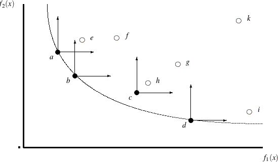
A Pareto-optimal set contains only nondominated solutions. In Figure 3.2, a Pareto-optimal frontier is plotted with respect to minimization objectives ![]() and
and ![]() along with a corresponding population of 10 points that are plotted in the objective space. In this example, point
along with a corresponding population of 10 points that are plotted in the objective space. In this example, point ![]() dominates
dominates ![]() ,
, ![]() dominates
dominates ![]() ,
, ![]() dominates
dominates ![]() , and
, and ![]() dominates
dominates ![]() . Although
. Although ![]() is not dominated by any other point in the population, it has not yet converged to the true Pareto-optimal frontier. Thus
there exist points in a neighborhood of
is not dominated by any other point in the population, it has not yet converged to the true Pareto-optimal frontier. Thus
there exist points in a neighborhood of ![]() that have smaller values of
that have smaller values of ![]() and
and ![]() .
.
In the constrained case, a point ![]() is dominated by a point
is dominated by a point ![]() if
if ![]() >
> ![]() and
and ![]() <
< ![]() , where
, where ![]() denotes the maximum constraint violation at point
denotes the maximum constraint violation at point ![]() and FEASTOL=
and FEASTOL=![]() thus feasibility takes precedence over objective function values.
thus feasibility takes precedence over objective function values.
Genetic algorithms enable you to attack multiobjective problems directly in order to evolve a set of Pareto-optimal solutions
in one run of the optimization process instead of solving multiple separate problems. In addition, local searches in neighborhoods
around nondominated points can be conducted to improve objective function values and reduce crowding. Because the number of
nondominated points that are encountered might be greater than the total population size, PROC OPTLSO stores nondominated
points in an archived set ![]() ; you can specify the PARETOMAX= option to control the size of this set.
; you can specify the PARETOMAX= option to control the size of this set.
Although it is difficult to verify directly that a point lies on the true Pareto-optimal frontier without using derivatives,
convergence can indirectly be measured by monitoring movement of the population with respect to ![]() , the current set of nondominated points. A number of metrics for measuring convergence in multiobjective evolutionary algorithms
have been suggested, such as the generational distance by Van Veldhuizen (1999), the inverted generational distance by Coello Coello and Cruz Cortes (2005), and the averaged Hausdorff distance by Schütze et al. (2012). PROC OPTLSO uses a variation of the averaged Hausdorff distance that is extended for general constraints.
, the current set of nondominated points. A number of metrics for measuring convergence in multiobjective evolutionary algorithms
have been suggested, such as the generational distance by Van Veldhuizen (1999), the inverted generational distance by Coello Coello and Cruz Cortes (2005), and the averaged Hausdorff distance by Schütze et al. (2012). PROC OPTLSO uses a variation of the averaged Hausdorff distance that is extended for general constraints.
Distance between sets is computed in terms of the distance between a point and a set, which in turn is defined in terms of
the distance between two points. The distance measure used by PROC OPTLSO for two points ![]() and
and ![]() is calculated as
is calculated as
where ![]() denotes the maximum constraint violation at point x. Then the distance between a point
denotes the maximum constraint violation at point x. Then the distance between a point ![]() and a set
and a set ![]() is defined as
is defined as
Let ![]() denote the set of all nondominated points within the current population at the start of generation
denote the set of all nondominated points within the current population at the start of generation ![]() . Let
. Let ![]() denote the set of all nondominated points at the start of generation
denote the set of all nondominated points at the start of generation ![]() . At the beginning of each generation,
. At the beginning of each generation, ![]() is always satisfied. Then progress made during iteration
is always satisfied. Then progress made during iteration ![]() +
+![]() is defined as
is defined as
Because ![]() whenever
whenever ![]() , the preceding sum is over the set of points in the population that move from a status of nondominated to dominated. In this
case, the progress made is measured as the distance to the nearest dominating point.
, the preceding sum is over the set of points in the population that move from a status of nondominated to dominated. In this
case, the progress made is measured as the distance to the nearest dominating point.