The GA Procedure
- Overview
-
Getting Started

-
Syntax
PROC GA Statement ContinueFor Call Cross Call Dynamicarray Call EvaluateLC Call GetDimensions Call GetObjValues Call GetSolutions Call Initialize Call MarkPareto Call Mutate Call Objective Function PackBits Call Programming Statements ReadChild Call ReadCompare Call ReadMember Call ReadParent Call ReEvaluate Call SetBounds Call SetCompareRoutine Call SetCross Call SetCrossProb Call SetCrossRoutine Call SetElite Call SetEncoding Call SetFinalize Call SetMut Call SetMutProb Call SetMutRoutine Call SetObj Call SetObjFunc Call SetProperty Call SetSel Call SetUpdateRoutine Call ShellSort Call Shuffle Call UnpackBits Function UpdateSolutions Call WriteChild Call WriteMember Call
-
Details
Using Multisegment Encoding Using Standard Genetic Operators and Objective Functions Defining a User Fitness Comparison Routine Defining User Genetic Operators Defining a User Update Routine Defining an Objective Function Defining a User Initialization Routine Specifying the Selection Strategy Incorporating Heuristics and Local Optimizations Handling Constraints Optimizing Multiple Objectives
-
Examples
- References
Example 3.3 Quadratic Objective with Linear Constraints, Using Bicriteria Approach
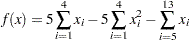
This example (Floudas and Pardalos 1992) illustrates the bicriteria approach to handling constraints. The problem has nine linear constraints and a quadratic objective function.
Minimize
 |
subject to
 |
and
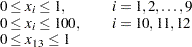 |
In this example, the linear constraint coefficients are specified in the SAS data set lincon and passed to the GA procedure with the MATRIX1= option. The upper and lower bounds are specified in the bounds data set specified with a DATA1= option, which creates the array variables upper and lower, matching the variables in the data set.
/* Input linear constraint matrix */
data lincon;
   input A1-A13 b;
   datalines;
 2  2  0  0  0  0  0  0  0  1  1  0  0 10
 2  0  2  0  0  0  0  0  0  1  0  1  0 10
 2  0  2  0  0  0  0  0  0  0  1  1  0 10
-8  0  0  0  0  0  0  0  0  1  0  0  0  0
 0 -8  0  0  0  0  0  0  0  0  1  0  0  0
 0  0 -8  0  0  0  0  0  0  0  0  1  0  0
 0  0  0 -2 -1  0  0  0  0  1  0  0  0  0
 0  0  0  0  0 -2 -1  0  0  0  1  0  0  0
 0  0  0  0  0  0  0 -2 -1  0  0  1  0  0
;

/* Input lower and upper bounds */
data bounds;
   input lower upper;
   datalines;
0  1
0  1
0  1
0  1
0  1
0  1
0  1
0  1
0  1
0  100
0  100
0  100
0  1
;
proc ga lastgen = out matrix1 = lincon
        seed = 12345 data1 = bounds;
Note also that the LASTGEN= option is used to designate a data set to store the final solution generation.
In the following statements, the solution encoding is specified, and a user function is defined and designated as the objective function.
call SetEncoding('R13R3');
nvar = 13;
ncon = 9;
function quad(selected[*], matrix1[*,*], nvar, ncon);

  array x[1] /nosym;

  array r[3] /nosym;

  array violations[1] /nosym;

  call dynamic_array(x, nvar);

  call dynamic_array(violations, ncon);

  call ReadMember(selected,1,x);

  sum1 = 0;

  do i = 1 to 4;

    sum1 + x[i] - x[i] * x[i];

  end;

  sum2 = 0;

  do i = 5 to 13;

    sum2 + x[i];

  end;

  obj = 5 * sum1 - sum2;

  call EvaluateLC(matrix1,violations,sumvio,selected,1);

  r[1] = obj;

  r[2] = sumvio;

  call WriteMember(selected,2,r);

  return(obj);

endsub;

call SetObjFunc('quad',0);
The SetEncoding call specifies two real-valued segments. The first segment, R13, holds the 13 variables, and the second segment, R3, holds the two objective criteria and the marker for Pareto optimality. As described in the section Defining an Objective Function, the first parameter of the objective function is a numeric array that designates which member of the solution population is to be evaluated. When the quad function is called by the GA procedure during the optimization process, the matrix1, nvar, and ncon parameters receive the values of the corresponding global variables; nvar is set to the number of variables, and ncon is set to the number of linear constraints. The function computes the original objective as the first objective criterion, and the magnitude of constraint violation as the second. With the first dynamic_array call, it allocates a working array, x, large enough to hold the number of variables, and a second array, violations, large enough to tabulate each constraint violation. The ReadMember call fills x with the elements of the first segment of the solution, and then the function computes the original objective  . The EvaluateLC call is used to compute the linear constraint violation. The objective and sum of the constraint violations are then stored in the array r, and written back to the second segment of the solution with the WriteMember call. Note that the third element of r is not modified, because that element of the segment is used to store the Pareto-optimality mark, which cannot be determined until all the solutions have been evaluated.
Next, a user routine is defined and designated to be an update routine. This routine is called once at each iteration, after all the solutions have been evaluated with the quad function. The following program illustrates this:
subroutine update(popsize);

  /* find pareto-optimal set */

  array minmax[3] /nosym (-1 -1 0);

  array results[1,1] /nosym;

  array scratch[1] /nosym;

  call dynamic_array(scratch, popsize);

  call dynamic_array(results,popsize,3);

  /* read original and constraint objectives, stored in

   * solution segment 2, into array */

  call GetSolutions(results,popsize,2);

  /* mark the pareto-optimal set */

  call MarkPareto(scratch, npareto,results, minmax);

  /* transfer the results to the solution segment */

  do i = 1 to popsize;

    results[i,3] = scratch[i];

  end;

  /* write updated segment 2 back into solution population */

  call UpdateSolutions(results,popsize,2);

  /* Set Elite parameter to preserve the first 15 pareto-optimal

   * solutions */

  if npareto < 16 then

     call SetElite(npareto);

  else

     call SetElite(15);

endsub;

call SetUpdateRoutine('update');
This subroutine has one parameter, popsize, defined within the GA procedure, which is expected to be the population size. The working arrays results, scratch, and minmax are declared. The minmax array is to be passed to a MarkPareto call, and is initialized to specify that the first two elements (the original objective and constraint violation) are to be minimized and the third element is not to be considered. The results and scratch arrays are then dynamically allocated to the dimensions required by the population size.
Next, the results array is filled with the second segment of the solution population, with the GetSolutions call. The minmax and results arrays are passed as inputs to the MarkPareto call, which returns the number of Pareto optimal solutions in the npareto variable. The MarkPareto call also sets the elements of the scratch array to 1 if the corresponding solution is Pareto-optimal, and to 0 otherwise. The next loop then records the results in the scratch array in the third column of the results array, effectively marking the Pareto-optimal solutions. The updated solution segments are written back to the population with the UpdateSolutions call.
The final step in the update routine is to set the elite selection parameter to guarantee the survival of at least a minimum of 15 of the fittest (Pareto-optimal) solutions through the selection process.
With the following statements, a routine is defined and designated as a fitness comparison routine with a SetCompareRoutine call. This routine works in combination with the update routine to evolve the solution population toward Pareto optimality and constraint satisfaction.
function paretocomp(selected[*]);

  array member1[3] /nosym;

  array member2[3] /nosym;

  call ReadCompare(selected,2,1, member1);

  call ReadCompare(selected,2,2, member2);

  /* if one member is in the pareto-optimal set

   * and the other is not, then it is the

   * most fit */

  if(member1[3] > member2[3]) then

     return(1);

  if(member2[3] > member1[3]) then

     return(-1);

  /* if both are in the pareto-optimal set, then

   * the one with the lowest constraint violation

   * is the most fit */

  if(member1[3] = 1) then do;

     if member1[2] <= member2[2] then

        return(1);

     return( -1);

  end;

  /* if neither is in the pareto-optimal set, then

   * take the one that dominates the other */

  if (member1[2] <= member2[2]) &

     (member1[1] <= member2[1]) then

     return(1);

  if (member2[2] <= member1[2]) &

     (member2[1] <= member1[1]) then

     return(-1);

  /* if neither dominates, then consider fitness to be

   * the same */

  return( 0);

endsub;

call SetSel('tournament', 'size', 2);

call SetCompareRoutine('paretocomp');
The PARETOCOMP subroutine is called in the selection process to compare the fitness of two competing solutions. The first parameter, selected, designates the two solutions to be compared.
The ReadCompare calls retrieve the second segments of the two solutions, where the objective criteria are stored, and writes the segments into the member1 and member2 arrays. The logic that follows first checks for the case where only one solution is Pareto optimal, and returns it. If both the solutions are Pareto optimal, then the one with the smallest constraint violation is chosen. If neither solution is Pareto optimal, then the dominant solution is chosen, if one exists. If neither solution is dominant, then no preference is indicated. After the function is defined, it is designated as a fitness comparison routine with the SetCompareRoutine call.
Next, subroutines are defined and designated as user crossover and mutation operators:
/* set up crossover parameters */

subroutine Cross1(selected[*], alpha);

   call Cross(selected,1,'twopoint', alpha);

endsub;

call SetCrossRoutine('Cross1',2,2);

alpha = 0.5;

call SetCrossProb(0.8);

/* set up mutation parameters */

subroutine Mut1(selected[*], delta[*]);

   call Mutate(selected,1,'delta',delta,1);

endsub;

call SetMutRoutine('Mut1');

array delta[13] /nosym (.5 .5 .5 .5 .5 .5 .5 .5 .5 10 10 10 .1);

call SetMutProb(0.05);
These routines execute the standard genetic operators twopoint for crossover and delta for mutation; see the section Using Standard Genetic Operators and Objective Functions for a description of each. The alpha and delta variables defined in the procedure are passed as parameters to the user operators, and the crossover and mutation probabilities are set with the SetCrossProb and SetMutProb calls.
At this point, the GA procedure is directed to initialize the first population and begin the optimization process:
/* Initialize first population */

call SetBounds(lower, upper);

popsize = 100;

call Initialize('DEFAULT',popsize);

call ContinueFor(500);

run;
First, the upper and lower bounds are established with values in the lower and upper array variables, which were set up by the DATA1= option in the PROC GA statement. The SetBounds call sets the bounds for the first segment, which is the default if none is specified in the call. The desired population size of 100 is stored in the popsize variable, so it will be passed to the update subroutine as the popsize parameter. The Initialize call specifies the default initialization, which generates values randomly distributed between the lower and upper bounds for the first encoding segment. Since no bounds were specified for the second segment, it is filled with zeros. The ContinueFor call sets the requested number of iterations to 500, and the RUN statement ends the GA procedure input and begins the optimization process. The output of the procedure is shown in Output 3.3.1.
| Bicriteria Constraint Handling Example |
| Objective |
|---|
| -14.99871988 |
| Solution | ||
|---|---|---|
| Segment | Element | Value |
| 1 | 1 | 1 |
| 1 | 2 | 0.9999997423 |
| 1 | 3 | 0.9999991741 |
| 1 | 4 | 0.9999997454 |
| 1 | 5 | 0.9999982195 |
| 1 | 6 | 1 |
| 1 | 7 | 0.9999674484 |
| 1 | 8 | 0.9999961238 |
| 1 | 9 | 0.9999691145 |
| 1 | 10 | 2.9999914332 |
| 1 | 11 | 2.9999103023 |
| 1 | 12 | 2.9988939259 |
| 1 | 13 | 1 |
| 2 | 1 | -14.99871988 |
| 2 | 2 | 0 |
| 2 | 3 | 1 |
The minimum value of is  at
at  .
.