Wavelet Analysis

Some Brief Mathematical Preliminaries
The discrete wavelet transform decomposes a function as a sum of basis functions called wavelets. These basis functions have
the property that they can be obtained by dilating and translating two basic types of wavelets known as the scaling function, or father wavelet  , and The mother wavelet
  . These translations and dilations are defined as follows:
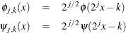
The index j defines the dilation or level while the index k defines the translate. Loosely speaking, sums of the  capture low frequencies and sums of the
  represent high frequencies in the data. More precisely, for any suitable function
  and for any
  ,
,
![\[ f(x)= \sum _ k c^{j_0}_ k \phi _{j_0,k}(x) + \sum _{j \geq j_0} \sum _ k d^ j_ k \psi _{j,k}(x) \]](images/imlug_waveletanalysis0008.png)
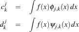
where the  and
and  are known as the scaling coefficients and the detail coefficients, respectively. For orthonormal wavelet families these coefficients
can be computed by
are known as the scaling coefficients and the detail coefficients, respectively. For orthonormal wavelet families these coefficients
can be computed by
The key to obtaining fast numerical algorithms for computing the detail and scaling coefficients for a given function is that there are simple recurrence relationships that enable you to compute the coefficients at level  from the values of the scaling coefficients at level j. These formulas are
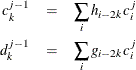
The coefficients  and
and  that appear in these formulas are called filter coefficients. The are determined by the father wavelet and they form a low-pass filter;
  and form a high-pass filter. The preceding sums are formally over the entire (infinite) range of integers. However, for wavelets
that are zero except on a finite interval, only finitely many of the filter coefficients are nonzero, and so in this case
the sums in the recurrence relationships for the detail and scaling coefficients are finite.
and form a high-pass filter. The preceding sums are formally over the entire (infinite) range of integers. However, for wavelets
that are zero except on a finite interval, only finitely many of the filter coefficients are nonzero, and so in this case
the sums in the recurrence relationships for the detail and scaling coefficients are finite.
Conversely, if you know the detail and scaling coefficients at level , then you can obtain the scaling coefficients at level j by using the relationship
![\[ c^ j_ k = \sum _ i h_{k-2i} c^{j-1}_ i + \sum _ i g_{k-2i}d^{j-1}_ i \]](images/imlug_waveletanalysis0017.png)
Suppose that you have data values
![\[ y_ k = f(x_ k), \qquad k=0,1,2,\cdots ,N-1 \]](images/imlug_waveletanalysis0018.png)
at  equally spaced points
  . It turns out that the values
  are good approximations of the scaling coefficients
  . Then, by using the recurrence formula, you can find
  and
and  ,
, 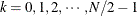 . The discrete wavelet transform of the
  at level
  consists of the
  scaling and detail coefficients at level . A technical point that arises is that in applying the recurrence relationships to finite data, a few values of the for
  or
or  might be needed. One way to cope with this difficulty is to extend the sequence to the left and right by using some specified boundary treatment.
Continuing by replacing the scaling coefficients at any level j by the scaling and detail coefficients at level j – 1 yields a sequence of N coefficients
![\[ \{ c^0_0,d^0_0,d^1_0,d^1_1,d^2_0,d^2_1,d^2_2,d^2_3,d^3_1,\ldots ,d^3_7,\ldots ,d^{J-1}_0,\ldots ,d^{J-1}_{N/2-1}\} \]](images/imlug_waveletanalysis0031.png)
This sequence is the finite discrete wavelet transform of the input data  . At any level the finite dimensional approximation of the function is
![\[ f(x)\approx \sum _ k c^{j_0}_ k \phi _{j_0,k}(x) + \sum _{j=j_0}^{J-1} \sum _ k d^ j_ k \psi _{j,k}(x) \]](images/imlug_waveletanalysis0033.png)