Nonlinear Optimization Examples

Constrained Betts Function

The linearly constrained Betts function (Hock and Schittkowski 1981) is defined as

$f(x) = 0.01 x_1^2 + x_2^2 - 100$

The boundary constraints are

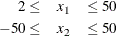
$\begin{eqnarray*} 2 \leq & x_1 & \leq 50 \\ -50 \leq & x_2 & \leq 50 \end{eqnarray*}$

The linear constraint is

$10x_1 - x_2 \geq 10$

The following code calls the NLPCG subroutine to solve the optimization problem. The infeasible initial point $x^0 = (-1,-1)$ is specified, and a portion of the output is shown in Figure 15.3.

proc iml;
start F_BETTS(x);
   f = .01 * x[1] * x[1] + x[2] * x[2] - 100.;
   return(f);
finish F_BETTS;

con = {  2. -50.  .   .,
        50.  50.  .   .,
        10.  -1. 1. 10.};
x = {-1. -1.};
optn = {0 2};
ods select ParameterEstimates LinCon ProblemDescription
    IterStart IterHist IterStop LinConSol;
call nlpcg(rc,xres,"F_BETTS",x,optn,con);
quit;

The NLPCG subroutine performs conjugate gradient optimization. It requires only function and gradient calls. The F_BETTS module represents the Betts function, and since no module is defined to specify the gradient, first-order derivatives are computed by finite-difference approximations. For more information about the NLPCG subroutine, see the section NLPCG Call. For details about the constraint matrix, which is represented by the CON matrix in the preceding code, see the section Parameter Constraints.

Figure 15.3: NLPCG Solution to Betts Problem

Optimization Start
Parameter Estimates
N	Parameter	Estimate	Gradient Objective Function	Lower Bound Constraint	Upper Bound Constraint
1	X1	6.800000	0.136000	2.000000	50.000000
2	X2	-1.000000	-2.000000	-50.000000	50.000000

Linear Constraints
1	59.00000	:		10.0000	<=	+	10.0000	*	X1	-	1.0000	*	X2

Parameter Estimates	2
Lower Bounds	2
Upper Bounds	2
Linear Constraints	1

Optimization Start
Active Constraints	0	Objective Function	-98.5376
Max Abs Gradient Element	2

Iteration	Restarts	Function Calls	Active Constraints	Objective Function	Objective Function Change	Max Abs Gradient Element	Step Size	Slope of Search Direction
1	0	3	0	-99.54682	1.0092	0.1346	0.502	-4.018
2	1	7	1	-99.96000	0.4132	0.00272	34.985	-0.0182
3	2	9	1	-99.96000	1.851E-6	0	0.500	-74E-7

Optimization Results
Iterations	3	Function Calls	10
Gradient Calls	9	Active Constraints	1
Objective Function	-99.96	Max Abs Gradient Element	0
Slope of Search Direction	-7.398365E-6

Optimization Results
Parameter Estimates
N	Parameter	Estimate	Gradient Objective Function	Active Bound Constraint
1	X1	2.000000	0.040000	Lower BC
2	X2	-1.24028E-10	0

Linear Constraints Evaluated at Solution
1		10.00000	=	-10.0000	+	10.0000	*	X1	-	1.0000	*	X2

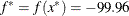Since the initial point $(-1,-1)$ is infeasible, the subroutine first computes a feasible starting point. Convergence is achieved after three iterations, and the optimal point is given to be $x^* = (2,0)$ with an optimal function value of $f^* = f(x^*) = -99.96$ . For more information about the printed output, see the section Printing the Optimization History.