Language Reference
FARMACOV Call
CALL FARMACOV (cov, d <*>, phi <*>, theta <*>, sigma <*>, p <*>, q <*>, lag );
The FARMACOV subroutine computes the autocovariance function for an autoregressive fractionally integrated moving average
(ARFIMA) model of the form ARFIMA( ).
).
The input arguments to the FARMACOV subroutine are as follows:
- d
-
specifies a fractional differencing order. The value of d must be in the open interval
 excluding zero. This input is required.
- phi
-
specifies an
 -dimensional vector that contains the autoregressive coefficients, where is the number of the elements in the subset of the AR order. The default is zero. All the roots of
  should be greater than one in absolute value, where
  is the finite-order matrix polynomial in the backshift operator B, such that
  .
.
- theta
-
specifies an
 -dimensional vector that contains the moving average coefficients, where is the number of the elements in the subset of the MA order. The default is zero.
- p
-
specifies the subset of the AR order. The quantity
is defined as the number of elements of phi.
If you do not specify p, the default subset is p
 .
.
For example, consider phi=0.5.
If you specify p=1 (the default), the FARMACOV subroutine computes the theoretical autocovariance function of an ARFIMA(
 ) process as
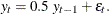
If you specify p=2, the FARMACOV subroutine computes the autocovariance function of an ARFIMA(
 ) process as
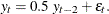
- q
-
specifies the subset of the MA order. The quantity
is defined as the number of elements of theta.
If you do not specify q, The default subset is q
 .
.
The usage of q is the same as that of p.
- lag
-
specifies the length of lags, which must be a positive number. The default is lag=12.
The FARMACOV subroutine returns the following value:
- cov
-
is a lag
 vector that contains the autocovariance function of an ARFIMA() process.
As an example, consider the following ARFIMA( ) process:
![\[ (1-0.5B)(1-B)^{0.3}y_ t = (1+0.1B){\epsilon }_ t \]](images/imlug_langref0291.png)
In this process,  . The following statements compute the autocovariance of this process:
d = 0.3;
phi = 0.5;
theta = -0.1;
sigma = 1.2;
call farmacov(cov, d, phi, theta, sigma) lag=5;
print cov;
Figure 25.130: Autocovariance of an ARFIMA Process
For  , the series
  represented as
  is a stationary and invertible ARFIMA(
 ) process with the autocovariance function
![\[ \gamma _ k = {\mbox E}(y_{t}y_{t-k}) = { {(-1)^ k \Gamma (-2d+1)} \over {\Gamma (k-d+1)\Gamma (-k-d+1) }} \]](images/imlug_langref0297.png)
and the autocorrelation function
![\[ \rho _ k = {\gamma _ k \over \gamma _0} = {{ \Gamma (-d+1)\Gamma (k+d)} \over {\Gamma (d)\Gamma (k-d+1) }} \sim { \Gamma (-d+1) \over {\Gamma (d)}} k^{2d-1}, ~ ~ k\rightarrow \infty \]](images/imlug_langref0298.png)
Notice that  decays hyperbolically as the lag increases, rather than showing the exponential decay of the autocorrelation function of
a stationary ARMA(
decays hyperbolically as the lag increases, rather than showing the exponential decay of the autocorrelation function of
a stationary ARMA( ) process.
For  , the series is a stationary and invertible ARFIMA() process represented as
![\[ \phi (B)(1-B)^ dy_ t = \theta (B){\epsilon }_ t \]](images/imlug_langref0301.png)
where  and
and  and
and  is a white noise process; all the roots of the characteristic AR and MA polynomial lie outside the unit circle.
Let  , so that
  follows an ARFIMA() process; let
  , so that
  follows an ARMA() process; let
  be the autocovariance function of
  and
and  be the autocovariance function of
  .
.
Then the autocovariance function of  is as follows:
![\[ \gamma _ k = \sum _{j=-\infty }^{j=\infty } \gamma _ j^ z\gamma _{k-j}^ x \]](images/imlug_langref0313.png)
The explicit form of the autocovariance function of is given by Sowell (1992).